# deep_learning
**Repository Path**: aidysun/deep_learning
## Basic Information
- **Project Name**: deep_learning
- **Description**: Learning notes and self assignments implementation
- **Primary Language**: Python
- **License**: MIT
- **Default Branch**: master
- **Homepage**: None
- **GVP Project**: No
## Statistics
- **Stars**: 0
- **Forks**: 0
- **Created**: 2020-11-05
- **Last Updated**: 2020-12-19
## Categories & Tags
**Categories**: Uncategorized
**Tags**: None
## README
# Deep Neural Network
- [Binary Classification / Logistic Regression](#binary-classification--logistic-regression)
- [Steps for developing a neural network](#steps-for-developing-a-neural-network)
- [Bias & Variance](#bias--variance)
- [Terminologies](#terminologies)
- [Activation Functions](#activation-functions)
- [Derivatives](#derivatives)
- [Backward Propagation](#backward-propagation)
- [Loss / Cost Function](#loss--cost-function)
- [Loss](#loss)
- [Parameters Initialization](#parameters-initialization)
- [Normalization](#normalization)
- [Cost \(gradients\)](#cost-gradients)
- [Regularization](#regularization)
- [Gradient Checking](#gradient-checking)
- [Mini-batch](#mini-batch)
- [Hyper-parameters tuning](#hyper-parameters-tuning)
- [Convolutional Neural Network](#convolutional-neural-network)
- [Residual Networks \(ResNets\)](#residual-networks-resnets)
- [Inception Networks](#inception-networks)
- [Data Argumentation](#data-argumentation)
- [Transfer Learning](#transfer-learning)
- [Data vs. Hand-engineering](#data-vs-hand-engineering)
- [Object Detection](#object-detection)
- [NN Architectures](#nn-architectures)
- [Face Recognition](#face-recognition)
- [Neural Style Transfer](#neural-style-transfer)
- [Recurrent Neural Network \(RNN\)](#recurrent-neural-network-rnn)
- [LTSM \(long short-term memory\)](#ltsm-long-short-term-memory)
- [BRNN \(Bidirectional RNN\)](#brnn-bidirectional-rnn)
* Courses
1. Neural Networks and Deep Learning
2. Improving Deep Neural Networks: Hyperparameter tuning, Regularization and Optimization
3. Structuring Machine Learning Projects
4. Convolutional Neural Networks
5. Sequence Models
## Binary Classification / Logistic Regression
Lost is smaller is better.
```
Lost(yhat, y) = - (y * log(yhat) + (1-y) * log(1-yhat))
```
if y = 1, `Lost = -log(yhat)`, we want Lost to be small, then `log(yhat)` be large, then `yhat` be large
## Steps for developing a neural network
1. Reduce cost
* gradient reduce
* ...
2. Prevent over-fitting
* more data (data augmentation)
* regularization
* drop-out
* ...
## Bias & Variance
| | high variance | high bias | high var & bias| low var & bias|
|:--|:--:|:--:|:--:|:--:|
|train set error: | 1% | 15% | 19% | 0.9% |
|dev set error: | 11% | 16% |30% | 1% |
1. High bias (training set performance)
- larger network
- more layers
- more units
- training longer
- (NN architecture search)
2. High variance (dev set performance)
- more training data
- regularization
- L2
- Dropout
- (NN architecture search)
## Terminologies
- Epoch : **entire** dataset is passed forward and backward through the neural network only ONCE
- **entire** means the whole dataset may not be passed to network at the same time, like mini-batch
- Batch Size: number of training examples in a single batch
- Iterations: the number of batches needed to complete one epoch
- `#iteration = #examples / #batch-size`
- Exploding gradients
- parameters go large, even NaN
- solution: gradient clipping
## Activation Functions
Activation function (a.k.a. transfer function) maps the resulting values into range. E.g. (0, 1) or (-1, 1).
Activation functions can be basically divided to *Linear* and *Non-linear* activation functions.
[Common Activation Functions Cheatsheet](images/common_activation_functions_cheatsheet.png)
* ReLU (Rectified Linear Unit)
- first choice when you are not sure which activation function to use
- result range [0, +infinity)
```python
g(z) = a = max(0, z)
g'(z) = 0 [when z < 0]; 1 [when z >= 0] # (A > 0)
# dZ = dA * g'(z) = np.multiply(dA, np.int64(A > 0))
```
* Leaky ReLU
- little better than ReLU
- result range (-infinity, +infinity)
```python
g(z) = a = max(0.01 * z, z)
g'(z) = 0.01 [when z < 0]; 1 [when z >= 0]
```
* tanh
- better than sigmoid, shift version of sigmoid
- result range (-1, 1)
```python
g(z) = a = (e[z] - e[-z]) / (e[z] + e[-z])
g'(z) = (1 - a.power(2))
```
* sigmoid
- rearly used except the output layer when output range between `{0, 1}`
- result range (0, 1)
```python
g(z) = a = 1 / (1 + e.power(-z)) = 1 / (1 + np.exp(-z))
g'(z) = a * (1 - a)
# da = -(y/a) + (1-y)/(1-a)
# dz = da * g'(z) = a * (1-a) * (-y/a + (1-y)/(1-a)) = a - y
```
- `sigmoid` is for two-class logistic regression while `softmax` is for multipclass logistic regression
## Derivatives
**gradient (also called the slope or derivative)**
Derivative is the slope of the function graph. `slope = height/weight` where `weight` is the change of input,
`height` is the change of output.
```
d(a^2) = 2a
d(a^3) = 3a^2
dlog(a) = 1/a
```
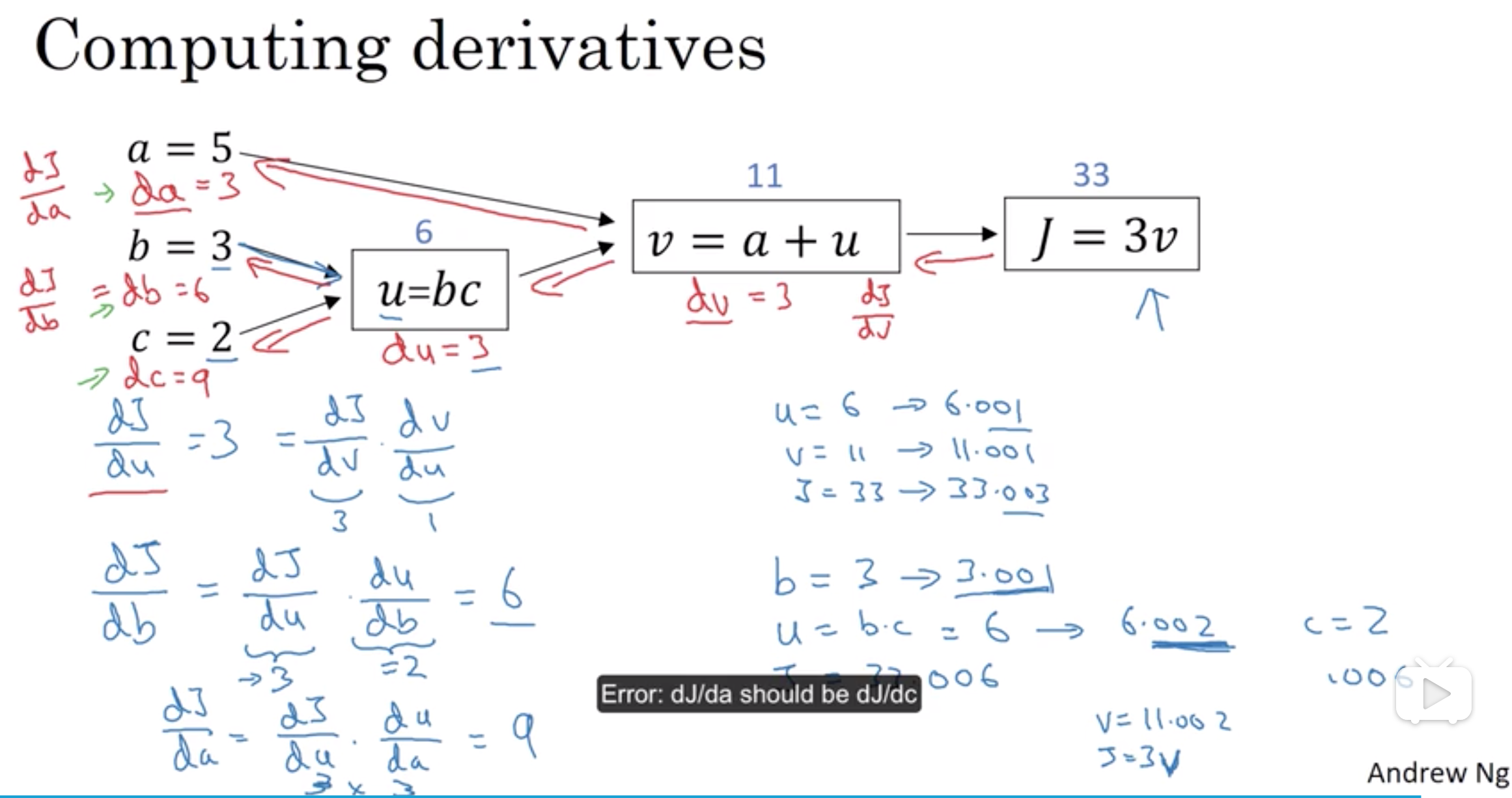
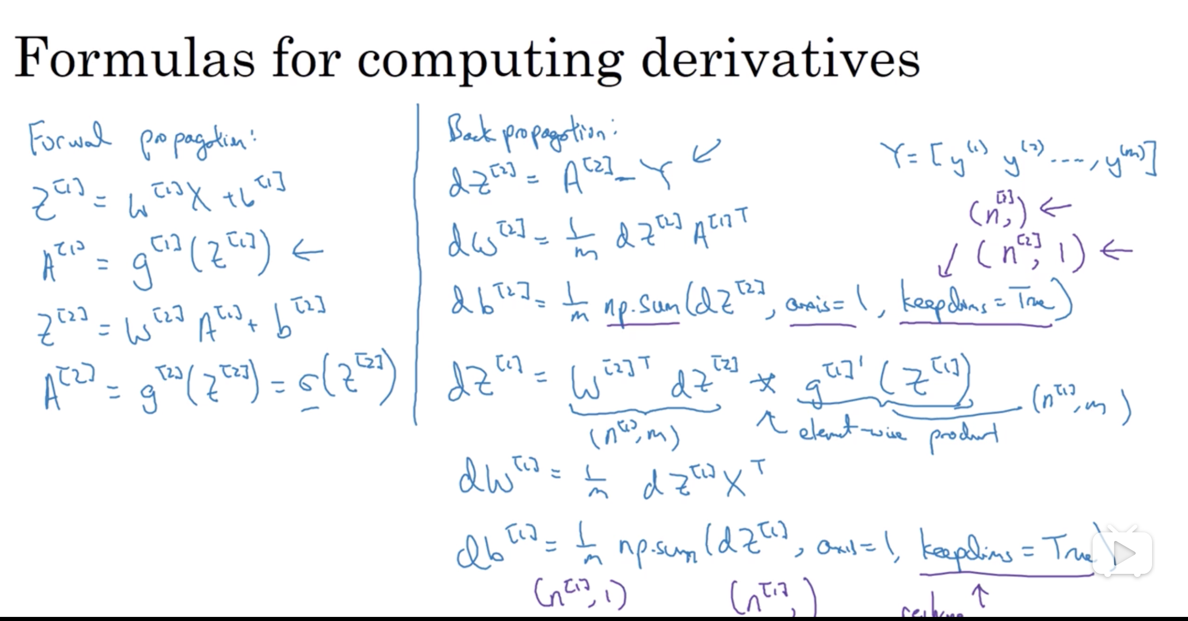
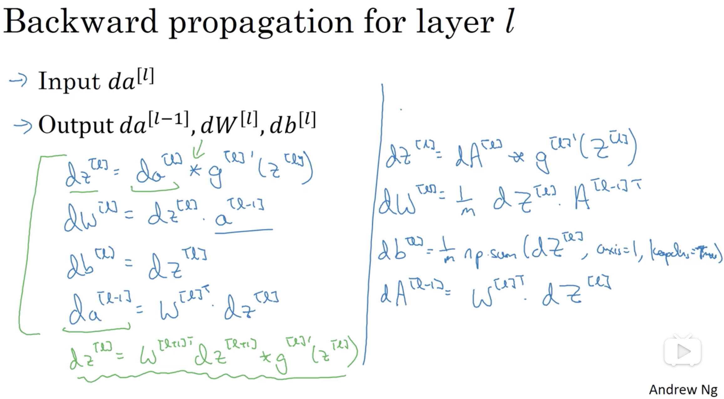
## Backward Propagation
**Note:** np.dot() performs a matrix-matrix or matrix-vector multiplication. This is different from np.multiply()
and the * operator (which is equivalent to .* in Matlab/Octave), which performs an element-wise multiplication.
```python
dA[l] = np.dot(W[l+1].T, dZ[l+1])
dZ[l] = np.multiply(dA[l], g[l]'(Z))
dW[l] = np.dot(dZ[l], A[l-1].T) / m
db[l] = np.sum(dZ[l], axis = 1, keepdims = True) / m
# dZ[l] = dA[l] * g[l]'(Z[l]) = np.multiply(np.dot(W[l+1].T, dZ[l+1]), g[l]'(Z[l]))
```
 ## Loss / Cost Function
### Loss
The loss is used to evaluate the performance of your model. The bigger your loss is, the more different your predictions ( ŷ y^ ) are from the true values ( yy ). In deep learning, you use optimization algorithms like Gradient Descent to train your model and to minimize the cost.
* L1 loss
```python
def L1(yhat, y):
l = np.sum(np.abs(yhat - y))
return l
```
* L2 loss
```python
def L2(yhat, y):
return np.dot(yhat-y, yhat-y)
```
## Parameters Initialization
- `W > I` could cause exploding, or vanishing when `W < I`
Init W with zeros will cause all layers do the same thing, cost is not changed (fail to break symmetry)
Init W with random big numbers can break symmetry, but it will slow down optimization algorithm (high loss for wrong predict)
**NOTE:** do not initialize parameters too large!
```python
# *He initialization* works well for networks with ReLU activations.
W[l] = np.random.rand(layers_dims[l], layer_dims[l-1]) * np.sqrt(2 / layer_dims[l-1])
# Xavier initialization is multiply np.sqrt(1 / (n-1))
```
## Normalization


`softmax` function is a normalization function.
```python
def softmax(x):
x_exp = np.exp(x)
exp_sum = np.sum(x_exp, axis = 1, keepdims = True)
sm = x_exp / exp_sum
return sm
```
- Regression
```python
means = X[i].sum() / m
X = X - means
variances = (np.sum(np.power(X[i], 2)) / m
X = X / variances
```
- Batch Normalization (BN)
- Input norm can reduce the affect of distribution difference of input data
- Same as above, normalization between layers can make layers more independently
- which means less effect when previous output changes
- BN has slight regularization effect, similar to dropout
- Can use bigger learning rate
- Batch norm affect batch-size during training, but when predecting, it may just one input
- running average
```python
# for layer l, Z_l.shape = (l, m)
means = (Z_i.sum()) / m
variance = np.sum(np.power(Z_i, 2)) / m
Z_i_norm = (Z_i - means) / (np.sqrt(variance + epsilon))
Z_i_final = gamma * Z_i_norm + beta
```
## Cost (gradients)
```python
# cross_entropy_cost
J(W, b) = - (y * log(a) + (1-y) * log(1-a)) / m
```
## Regularization
* To reduce/prevent over-fitting / variance issue.
* Drive weights to lower values.
* Hurts training set performance but gives better test accuracy.
1. L2-regularization
- Could be used at the beginning.
- An alternate to early stopping.
- relies on the assumption that *a model with smaller weights is simpler than model with large weights*
- forward (cost) and backward (W update) propagations both need change
- weight decay
```python
# cost with L2 regularization
L2_regularization_cost = (lambda / 2m)* (sum(W1^2) + sum(W2^2) + ... + sum(Wn^2))
J_regularization(W, b) = cross_entropy_cost + L2_regularization_cost
# d(L2_regularization_cost) / dW = (lambda / m) * W
# dW[l] = np.dot(dZ[l], A[l-1].T) / m
dW_regularization[l] = dW[l]+ (lambda / m) * W[l]
# It's called 'weight decay' because this makes weights end up smaller. Why?
# Because when updating W with dW, (learning_rate * lambda / m) is smaller than 1.
# Therefore, updated W[l] is smaller than non-regularization.
W[l] = W[l] - learning_rate * dW_regularization[l]
= (1 - learning_rate * lambda / m) * W[l] - learning_rate * dW[l]
```
2. Drop-out
- Should be used when the NN has overfitting issue.
- With dropout, the neurons become less sensitive to the activation. This would prevent overfitting (high variance).
- Intuition: cannot rely on any one feature, so have to spread out weights (shrink weights).
- Dropout should be used ONLY in training, not testing.
- Dropout apply to both forward and backward propagation.
- Shown to be an adaptive form without regularization. But drop-out has a similar effect to L2-regularization.
```python
# forward propagation
D[l] = (np.random.rand(A[l].shape) < keep_prob)
# by dividing keep_prob to keep the same expected value for activations as without dropout (inverted drop-out)
A[l] = (A[l] * D[l]) / keep_prob
# backward propagation
dA[l] = (dA[l] * D[l]) / keep_prob
```
## Gradient Checking
```python
J+ = forward_propagation(W+)
J- = forward_propagation(W-)
grad_approx = (J+ - J-) / (2 * epsilon)
diff = (grad - grad_approx).norm / (grad.norm() + grad_approx.norm())
```
## Mini-batch
- Parameters are adjusted for each epoch X
* Momentum
- smooth out the update of parameters in mini-batch
```python
v[dW(i)] = beta * v[dW(i)] + (1-beta)grads[dW(i)] // default beta = 0.9 is reasonable
parameters[W(i)] = parameters[W(i)] - learning_rate * v[dW(i)]
// same for db
```
* Adom
```pyton
v[dW_i] = beta1 * v[dW_i] + (1 - beta1) * dW_i
v_correct[dW_i] = v[dW_i] / (1 - np.power(beta1, i))
s[dW_i] = beta2 * s[dW_i] + (1 - beta2) * np.power(dW_i, 2)
s_correct[dW_i] = s[dW_i] / (1 - np.power(beta2, i))
W_i = W_i - learning_rate * (v_correct[dW_i] / (np.sqrt(s_correct[dW_i]) + epsilon))
// same for db
```
## Hyper-parameters tuning
- Scale to pick hyper-parameters
- linear way is not the best because the impact in different range is quite different
E.g. beta in momentum, the more beta close to 1, the more impact with tiny changes. (0.9 ~ 0.9005 comparing to 0.999 ~ 0.9995)
```python
# linear r [-4, 0]
r = -4 * np.random.rand()
# alpha is in [0.0001, 1]
alpha = np.power(10, r)
# liner r [-3, -1]
r = np.random.uniform(-3, -1)
# beta is in [0.9, 0.999]
beta = 1 - np.power(10, r)
```
## Convolutional Neural Network
- Why Convolutions
- Parameter sharing: a feature detector (filter) is shared
- (e.g. edge detector filter that is useful in part of image is also useful for another part of image)
- much less paramters than MLP to learn
- Sparsity of connections: in each layer, each output value only depends on a small number of input (conv layer with filter)
- Convolution operation
**NOTE:** symbol `*` in this section is convolution operation, not multiply and numpy.dot()
- cross-correlation (flipping filter) may not be mentioned
- input * filter = output
- `[n, n] * [f, f] = [(n-f+1), (n-f+1)]`
- problems:
- vanishing (because output is getting smaller)
- unfair to edge pixels
- solution: **padding**
- why filter usually is odd?
- easy for padding
- central pixel ???
- stride
- output = `[((n - f + 2p)/s + 1), ((n - f + 2p)/s + 1)]`
- `floor()` rounding is used
- 1 by 1 conv layer
- NiN (Network in Network)
- 1 * 1 * n[c-pre] * n[c] (filter)
- change (increase/decrease/keep same) channel
- bottleneck layer - which can reduce the number of parameter without affecting performance (Google inception network)
- Pooling
- combine multiple neuron clusters into a single neuron
- `max` and `avg`
- shrink height and wight (1X1 conv layer can shrink channel)
- Fully connected
- non-convolution, same as multilayer perceptron network (MLP)
## Residual Networks (ResNets)
- Why
- lower learning speed with deeper networks, because of vanishing gradient (gradient decrease to zero quickly)
- deeper networks cause perforcement degrading
- Two main types of blocks
- Identity Block (input activation has the same dimension with output activation)
- Convolutional Block
- shortcut has Conv and BN to resize the input to be the same dimension of the output to be added with
## Inception Networks
- Paper "Going Deeper with Convolutions" by Szegedy
- same shape with different channels, concat them as one layer (Filter concatenation)
- GooLeNet
## Data Argumentation
- Mirroring
- Random Cropping
- Rotation
- Shearing
- Local Warping
- Color Shifting
## Transfer Learning
- Init with pretrained models/parameters
## Data vs. Hand-engineering
- Data amount
- Speech Recognition > Image Recognition > Object Detection
## Object Detection
- Classification -> Object Localization -> Multiple Detection
- YOLO
- NMS _(non-maximum suppression)_
- Region Propose
- Sliding Windows
- R-CNN _(Reigions with CNN)_
- propose regions with algorithm *Seletive Search*
- then run a CNN on **each** of region proposals
- output is **bounding box**, not the shape of region
- Fast R-CNN
- perform *feature extraction* over image before proposing regions
- Faster R-CNN
- RPN _(Region Proposal Network)_
- Faster R-CNN = RPN + Fast R-CNN
- R-FCN _(Region-based Fully Convolutional Net)_
- SSD _(Single Shot Multibox Detector)_
- region preposing and classification were done in two seperate networks (CNN),
SSD does the two in a "single shot".
- it ignores the step of region proposing
- using NMS
## NN Architectures
- Feedforward networks, like cat/dog classification, samples have no
- RNN
- Recurrent Neural Network (时间递归)
- LSTM (long short-term memory)
- partially avoid vanishing gradient of RNN
- Recursive Neural Network (结构递归)
- Neural Network Attention
- less computation resource than RNN and LSTM
- avoid vanishing gradient
## Face Recognition
- Verification v.s. Recognition
- verification is 1:1 problem. verify input is the same as expected.
- recognition is 1:n problem.
- image -> CNN -> SoftMax -> output
- input data dependent
- e.g. CNN was trained with 100 persons, when the 101st person is added, CNN requires retraining
- Similarity function
- `if d(image1, image2) < threshold: same`
- Siamese Network (DeepFace)
-
## Loss / Cost Function
### Loss
The loss is used to evaluate the performance of your model. The bigger your loss is, the more different your predictions ( ŷ y^ ) are from the true values ( yy ). In deep learning, you use optimization algorithms like Gradient Descent to train your model and to minimize the cost.
* L1 loss
```python
def L1(yhat, y):
l = np.sum(np.abs(yhat - y))
return l
```
* L2 loss
```python
def L2(yhat, y):
return np.dot(yhat-y, yhat-y)
```
## Parameters Initialization
- `W > I` could cause exploding, or vanishing when `W < I`
Init W with zeros will cause all layers do the same thing, cost is not changed (fail to break symmetry)
Init W with random big numbers can break symmetry, but it will slow down optimization algorithm (high loss for wrong predict)
**NOTE:** do not initialize parameters too large!
```python
# *He initialization* works well for networks with ReLU activations.
W[l] = np.random.rand(layers_dims[l], layer_dims[l-1]) * np.sqrt(2 / layer_dims[l-1])
# Xavier initialization is multiply np.sqrt(1 / (n-1))
```
## Normalization


`softmax` function is a normalization function.
```python
def softmax(x):
x_exp = np.exp(x)
exp_sum = np.sum(x_exp, axis = 1, keepdims = True)
sm = x_exp / exp_sum
return sm
```
- Regression
```python
means = X[i].sum() / m
X = X - means
variances = (np.sum(np.power(X[i], 2)) / m
X = X / variances
```
- Batch Normalization (BN)
- Input norm can reduce the affect of distribution difference of input data
- Same as above, normalization between layers can make layers more independently
- which means less effect when previous output changes
- BN has slight regularization effect, similar to dropout
- Can use bigger learning rate
- Batch norm affect batch-size during training, but when predecting, it may just one input
- running average
```python
# for layer l, Z_l.shape = (l, m)
means = (Z_i.sum()) / m
variance = np.sum(np.power(Z_i, 2)) / m
Z_i_norm = (Z_i - means) / (np.sqrt(variance + epsilon))
Z_i_final = gamma * Z_i_norm + beta
```
## Cost (gradients)
```python
# cross_entropy_cost
J(W, b) = - (y * log(a) + (1-y) * log(1-a)) / m
```
## Regularization
* To reduce/prevent over-fitting / variance issue.
* Drive weights to lower values.
* Hurts training set performance but gives better test accuracy.
1. L2-regularization
- Could be used at the beginning.
- An alternate to early stopping.
- relies on the assumption that *a model with smaller weights is simpler than model with large weights*
- forward (cost) and backward (W update) propagations both need change
- weight decay
```python
# cost with L2 regularization
L2_regularization_cost = (lambda / 2m)* (sum(W1^2) + sum(W2^2) + ... + sum(Wn^2))
J_regularization(W, b) = cross_entropy_cost + L2_regularization_cost
# d(L2_regularization_cost) / dW = (lambda / m) * W
# dW[l] = np.dot(dZ[l], A[l-1].T) / m
dW_regularization[l] = dW[l]+ (lambda / m) * W[l]
# It's called 'weight decay' because this makes weights end up smaller. Why?
# Because when updating W with dW, (learning_rate * lambda / m) is smaller than 1.
# Therefore, updated W[l] is smaller than non-regularization.
W[l] = W[l] - learning_rate * dW_regularization[l]
= (1 - learning_rate * lambda / m) * W[l] - learning_rate * dW[l]
```
2. Drop-out
- Should be used when the NN has overfitting issue.
- With dropout, the neurons become less sensitive to the activation. This would prevent overfitting (high variance).
- Intuition: cannot rely on any one feature, so have to spread out weights (shrink weights).
- Dropout should be used ONLY in training, not testing.
- Dropout apply to both forward and backward propagation.
- Shown to be an adaptive form without regularization. But drop-out has a similar effect to L2-regularization.
```python
# forward propagation
D[l] = (np.random.rand(A[l].shape) < keep_prob)
# by dividing keep_prob to keep the same expected value for activations as without dropout (inverted drop-out)
A[l] = (A[l] * D[l]) / keep_prob
# backward propagation
dA[l] = (dA[l] * D[l]) / keep_prob
```
## Gradient Checking
```python
J+ = forward_propagation(W+)
J- = forward_propagation(W-)
grad_approx = (J+ - J-) / (2 * epsilon)
diff = (grad - grad_approx).norm / (grad.norm() + grad_approx.norm())
```
## Mini-batch
- Parameters are adjusted for each epoch X
* Momentum
- smooth out the update of parameters in mini-batch
```python
v[dW(i)] = beta * v[dW(i)] + (1-beta)grads[dW(i)] // default beta = 0.9 is reasonable
parameters[W(i)] = parameters[W(i)] - learning_rate * v[dW(i)]
// same for db
```
* Adom
```pyton
v[dW_i] = beta1 * v[dW_i] + (1 - beta1) * dW_i
v_correct[dW_i] = v[dW_i] / (1 - np.power(beta1, i))
s[dW_i] = beta2 * s[dW_i] + (1 - beta2) * np.power(dW_i, 2)
s_correct[dW_i] = s[dW_i] / (1 - np.power(beta2, i))
W_i = W_i - learning_rate * (v_correct[dW_i] / (np.sqrt(s_correct[dW_i]) + epsilon))
// same for db
```
## Hyper-parameters tuning
- Scale to pick hyper-parameters
- linear way is not the best because the impact in different range is quite different
E.g. beta in momentum, the more beta close to 1, the more impact with tiny changes. (0.9 ~ 0.9005 comparing to 0.999 ~ 0.9995)
```python
# linear r [-4, 0]
r = -4 * np.random.rand()
# alpha is in [0.0001, 1]
alpha = np.power(10, r)
# liner r [-3, -1]
r = np.random.uniform(-3, -1)
# beta is in [0.9, 0.999]
beta = 1 - np.power(10, r)
```
## Convolutional Neural Network
- Why Convolutions
- Parameter sharing: a feature detector (filter) is shared
- (e.g. edge detector filter that is useful in part of image is also useful for another part of image)
- much less paramters than MLP to learn
- Sparsity of connections: in each layer, each output value only depends on a small number of input (conv layer with filter)
- Convolution operation
**NOTE:** symbol `*` in this section is convolution operation, not multiply and numpy.dot()
- cross-correlation (flipping filter) may not be mentioned
- input * filter = output
- `[n, n] * [f, f] = [(n-f+1), (n-f+1)]`
- problems:
- vanishing (because output is getting smaller)
- unfair to edge pixels
- solution: **padding**
- why filter usually is odd?
- easy for padding
- central pixel ???
- stride
- output = `[((n - f + 2p)/s + 1), ((n - f + 2p)/s + 1)]`
- `floor()` rounding is used
- 1 by 1 conv layer
- NiN (Network in Network)
- 1 * 1 * n[c-pre] * n[c] (filter)
- change (increase/decrease/keep same) channel
- bottleneck layer - which can reduce the number of parameter without affecting performance (Google inception network)
- Pooling
- combine multiple neuron clusters into a single neuron
- `max` and `avg`
- shrink height and wight (1X1 conv layer can shrink channel)
- Fully connected
- non-convolution, same as multilayer perceptron network (MLP)
## Residual Networks (ResNets)
- Why
- lower learning speed with deeper networks, because of vanishing gradient (gradient decrease to zero quickly)
- deeper networks cause perforcement degrading
- Two main types of blocks
- Identity Block (input activation has the same dimension with output activation)
- Convolutional Block
- shortcut has Conv and BN to resize the input to be the same dimension of the output to be added with
## Inception Networks
- Paper "Going Deeper with Convolutions" by Szegedy
- same shape with different channels, concat them as one layer (Filter concatenation)
- GooLeNet
## Data Argumentation
- Mirroring
- Random Cropping
- Rotation
- Shearing
- Local Warping
- Color Shifting
## Transfer Learning
- Init with pretrained models/parameters
## Data vs. Hand-engineering
- Data amount
- Speech Recognition > Image Recognition > Object Detection
## Object Detection
- Classification -> Object Localization -> Multiple Detection
- YOLO
- NMS _(non-maximum suppression)_
- Region Propose
- Sliding Windows
- R-CNN _(Reigions with CNN)_
- propose regions with algorithm *Seletive Search*
- then run a CNN on **each** of region proposals
- output is **bounding box**, not the shape of region
- Fast R-CNN
- perform *feature extraction* over image before proposing regions
- Faster R-CNN
- RPN _(Region Proposal Network)_
- Faster R-CNN = RPN + Fast R-CNN
- R-FCN _(Region-based Fully Convolutional Net)_
- SSD _(Single Shot Multibox Detector)_
- region preposing and classification were done in two seperate networks (CNN),
SSD does the two in a "single shot".
- it ignores the step of region proposing
- using NMS
## NN Architectures
- Feedforward networks, like cat/dog classification, samples have no
- RNN
- Recurrent Neural Network (时间递归)
- LSTM (long short-term memory)
- partially avoid vanishing gradient of RNN
- Recursive Neural Network (结构递归)
- Neural Network Attention
- less computation resource than RNN and LSTM
- avoid vanishing gradient
## Face Recognition
- Verification v.s. Recognition
- verification is 1:1 problem. verify input is the same as expected.
- recognition is 1:n problem.
- image -> CNN -> SoftMax -> output
- input data dependent
- e.g. CNN was trained with 100 persons, when the 101st person is added, CNN requires retraining
- Similarity function
- `if d(image1, image2) < threshold: same`
- Siamese Network (DeepFace)
- distance(x1, x2) = ||f(x1) - f(x2)||2
- `f(x)` is encoding of input `x` (or the last FC layer vector)
- FaceNet
- triplet loss (anchor, positive, negative)
- training dataset should choose those triples `d(a, p)` close to `d(a, n)`
- Loss(A, P, N) = max(||f(A) - f(P)||2 - ||f(A) - f(N)||2 + alpha, 0)
## Neural Style Transfer
-
## Recurrent Neural Network (RNN)
- Why
- for problems that input and output have differect dimensions
- features are not shared across diff position (of text for example)
- Weekness
- only previous/earlier input are used to predection in one layer
- Bidirectional RNN (BRNN)
- vanishing gradient in deep network
- GRU (gated recurrent unit)
- a\ = g1(Waa a\ + Wax x\ + ba) # generally g1 = tanh/ReLu
- y_hat\ = g2(Wya a \ + by) # generally g2 = Sigmod
## LTSM (long short-term memory)
## BRNN (Bidirectional RNN)