# PixelCNN
**Repository Path**: hainan89/PixelCNN
## Basic Information
- **Project Name**: PixelCNN
- **Description**: 源出处:https://github.com/anordertoreclaim/PixelCNN
- **Primary Language**: Unknown
- **License**: Not specified
- **Default Branch**: master
- **Homepage**: None
- **GVP Project**: No
## Statistics
- **Stars**: 0
- **Forks**: 0
- **Created**: 2020-07-29
- **Last Updated**: 2020-12-19
## Categories & Tags
**Categories**: Uncategorized
**Tags**: None
## README
# PixelCNN
This repository is a PyTorch implementation of [PixelCNN](https://arxiv.org/abs/1601.06759) in its [gated](https://arxiv.org/abs/1606.05328) form.
The main goals I've pursued while doing it is to dive deeper into PyTorch and the network's architecture itself, which I've found both interesting and challenging to grasp. The repo might help someone, too!
A lot of ideas were taken from [rampage644](https://github.com/rampage644)'s, [blog](http://sergeiturukin.com). Useful links also include [this](https://wiki.math.uwaterloo.ca/statwiki/index.php?title=STAT946F17/Conditional_Image_Generation_with_PixelCNN_Decoders), [this](http://www.scottreed.info/files/iclr2017.pdf) and [this](https://github.com/kundan2510/pixelCNN).
# Model architecture
Here I am going to sum up the main idea behind the architecture. I won't go deep into implementation details and how convolutions work, because it would be too much text and visuals. Visit the links above in order to have a more detailed look on the inner workings of the architecture. Then come here for a summary :)
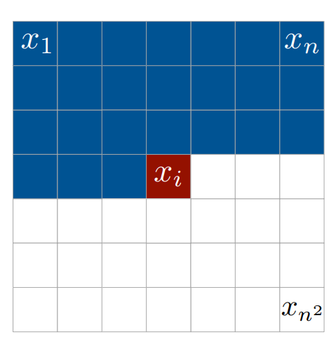
At first this architecture was an attempt to speed up the learning process of a RNN implementation of the same idea, which is a generative model that learns an explicit joint distribution of image's pixels by modeling it using simple chain rule:

The order is row-wise i.e. value of each pixel depends on values of all pixels above and to the left of it. Here is an explanatory image:
In order to achieve this property authors of the papers used simple masked convolutions, which in the case of 1-channel black and white images look like this:
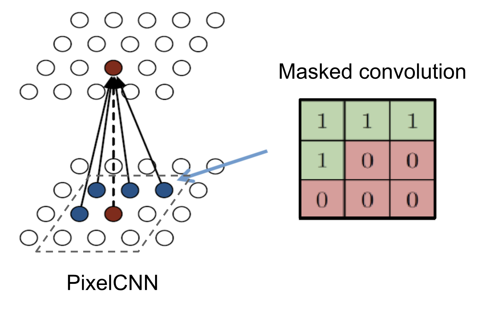
(i. e. convolutional filters are multiplied by this mask before being applied to images)
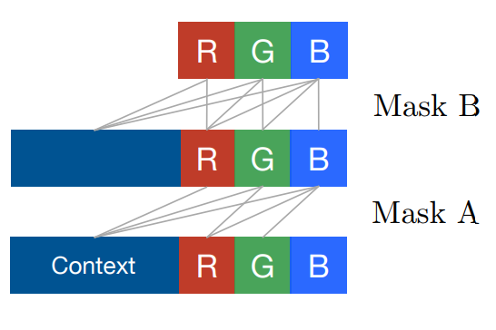
There are 2 types of masks: A and B. Masked convolution of type A can only see previously generated pixels, while mask of type B allows taking value of a pixel being predicted into consideration. Applying B-masked convolution after A-masked one preserves the causality, work it out! In the case of 3 data channels, types of masks are depicted on this image:
The problem with a simple masking approach was the blind spot: when predicting some pixels, a portion of the image did not influence the prediction. This was fixed by introducing 2 separate convolutions: horizontal and vertical. Vertical convolution performs a simple unmasked convolution and sends its outputs to a horizontal convolution, which performs a masked 1-by-N convolution. They also added conditioning on labels and gates in order to increase the predicting power of the model.
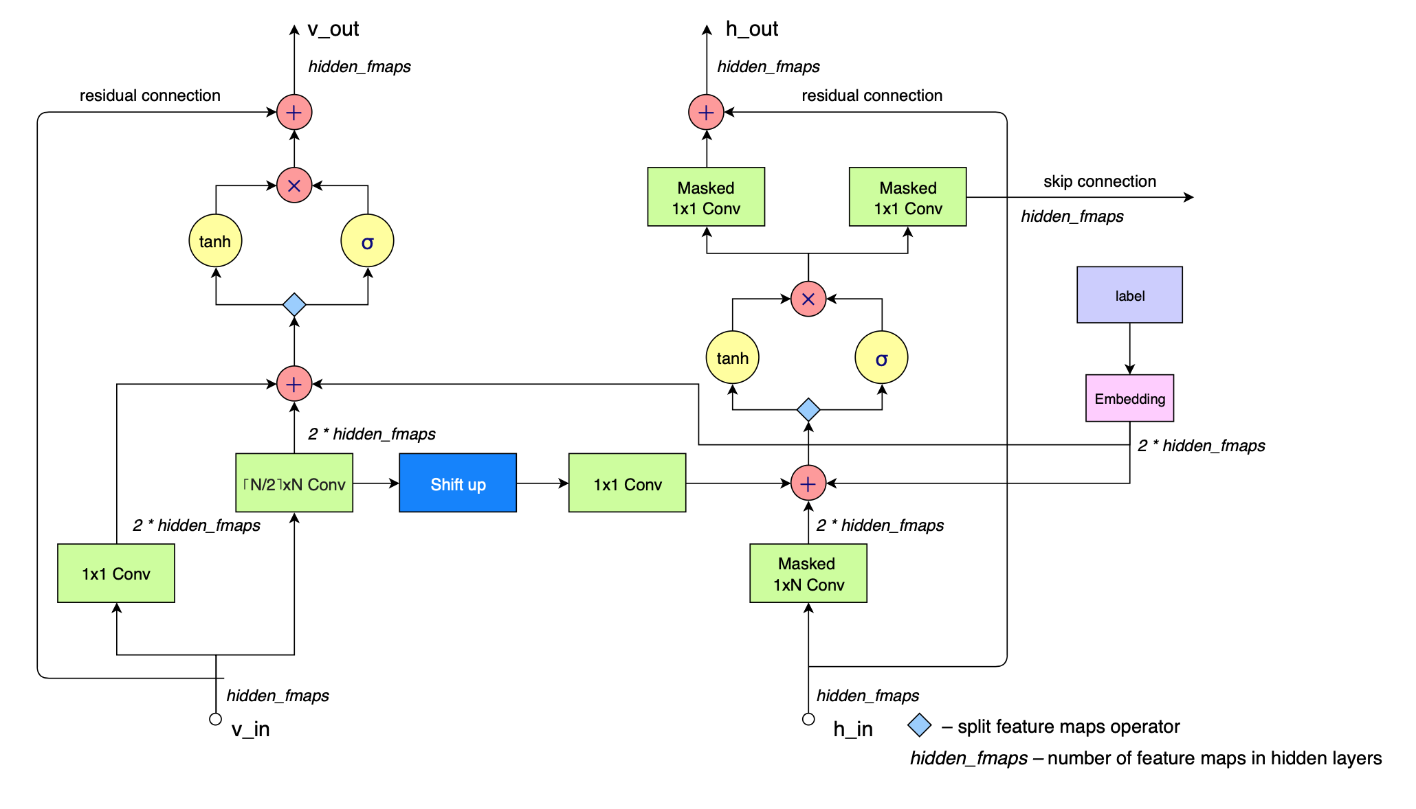
## Gated block
The main submodel of PixelCNN is a gated block, several of which are used in the network. Here is how it looks:
## High level architecture
Here is what the whole architecture looks like:

Causal block is the same as gated block, except that it has neither residual nor skip connections, its input is image instead of a tensor with depth of *hidden_fmaps*, it uses mask of type A instead of B of a usual gated block and it doesn't incorporate label bias.
Skip results are summed and ran through a ReLu – 1x1 Conv – ReLu block. Then the final convolutional layer is applied, which outputs a tensor that represents unnormalized probabilities of each color level for each color channel of each pixel in the image.
# Training and sampling
### Train
In order to train the model, use the `python train.py` command and set optional arguments if needed.
Model's state dictionary is saved to `model` folder by default. Samples which are generated during training are saved to `train_samples` folder by default.
Run `wandb login` in order to monitor hardware usage and each layer's gradients' distribution.
```
$ python train.py -h
usage: train.py [-h] [--epochs EPOCHS] [--batch-size BATCH_SIZE]
[--dataset DATASET] [--causal-ksize CAUSAL_KSIZE]
[--hidden-ksize HIDDEN_KSIZE] [--data-channels DATA_CHANNELS]
[--color-levels COLOR_LEVELS] [--hidden-fmaps HIDDEN_FMAPS]
[--out-hidden-fmaps OUT_HIDDEN_FMAPS]
[--hidden-layers HIDDEN_LAYERS]
[--learning-rate LEARNING_RATE] [--weight-decay WEIGHT_DECAY]
[--max-norm MAX_NORM] [--epoch-samples EPOCH_SAMPLES]
[--cuda CUDA]
PixelCNN
optional arguments:
-h, --help show this help message and exit
--epochs EPOCHS Number of epochs to train model for
--batch-size BATCH_SIZE
Number of images per mini-batch
--dataset DATASET Dataset to train model on. Either mnist, fashionmnist
or cifar.
--causal-ksize CAUSAL_KSIZE
Kernel size of causal convolution
--hidden-ksize HIDDEN_KSIZE
Kernel size of hidden layers convolutions
--color-levels COLOR_LEVELS
Number of levels to quantisize value of each channel
of each pixel into
--hidden-fmaps HIDDEN_FMAPS
Number of feature maps in hidden layer (must be
divisible by 3)
--out-hidden-fmaps OUT_HIDDEN_FMAPS
Number of feature maps in outer hidden layer
--hidden-layers HIDDEN_LAYERS
Number of layers of gated convolutions with mask of
type "B"
--learning-rate LEARNING_RATE, --lr LEARNING_RATE
Learning rate of optimizer
--weight-decay WEIGHT_DECAY
Weight decay rate of optimizer
--max-norm MAX_NORM Max norm of the gradients after clipping
--epoch-samples EPOCH_SAMPLES
Number of images to sample each epoch
--cuda CUDA Flag indicating whether CUDA should be used
```
### Sample
Sampling is performed similarly with `python sample.py`. Path to model's saved parameters must be defined.
Samples are saved to `samples/samples.png` by default.
```
$ python sample.py -h
usage: sample.py [-h] [--causal-ksize CAUSAL_KSIZE]
[--hidden-ksize HIDDEN_KSIZE] [--data-channels DATA_CHANNELS]
[--color-levels COLOR_LEVELS] [--hidden-fmaps HIDDEN_FMAPS]
[--out-hidden-fmaps OUT_HIDDEN_FMAPS]
[--hidden-layers HIDDEN_LAYERS] [--cuda CUDA]
[--model-path MODEL_PATH] [--output-fname OUTPUT_FNAME]
[--label LABEL] [--count COUNT] [--height HEIGHT]
[--width WIDTH]
PixelCNN
optional arguments:
-h, --help show this help message and exit
--causal-ksize CAUSAL_KSIZE
Kernel size of causal convolution
--hidden-ksize HIDDEN_KSIZE
Kernel size of hidden layers convolutions
--color-levels COLOR_LEVELS
Number of levels to quantisize value of each channel
of each pixel into
--hidden-fmaps HIDDEN_FMAPS
Number of feature maps in hidden layer
--out-hidden-fmaps OUT_HIDDEN_FMAPS
Number of feature maps in outer hidden layer
--hidden-layers HIDDEN_LAYERS
Number of layers of gated convolutions with mask of
type "B"
--cuda CUDA Flag indicating whether CUDA should be used
--model-path MODEL_PATH, -m MODEL_PATH
Path to model's saved parameters
--output-fname OUTPUT_FNAME
Name of output file (.png format)
--label LABEL, --l LABEL
Label of sampled images. -1 indicates random labels.
--count COUNT, -c COUNT
Number of images to generate
--height HEIGHT Output image height
--width WIDTH Output image width
```
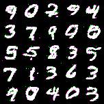
# Examples of samples
The biggest challenge is to make the network converge to a good set of parameters. I've experimented with hyperparameters and here are the results I've managed to obtain for N-way MNIST using different models.
Generally, in order for model to converge to a good set of parameters, one needs to go with a small learning rate (about 1e-4). I've also found that bigger kernel sizes in hidden layers work better.
A very simple model, `python train.py --epochs 2 --color-levels 2 --hidden-fmaps 21 --lr 0.002 --max-norm 2` (all others are default values), trained for just 2 epochs, managed to produce these samples on a binary MNIST:
`python train.py --lr 0.0002` (quite a simple model, too) produced these results:

A more complex model, `python train.py --color-levels 10 --hidden-fmaps 120 --out-hidden-fmaps 60 --lr 0.0002`, managed to produce these on a 10-way MNIST:
