# fft_pipeline_multimode
**Repository Path**: laifu1/fft_pipeline_multimode
## Basic Information
- **Project Name**: fft_pipeline_multimode
- **Description**: No description available
- **Primary Language**: Unknown
- **License**: Not specified
- **Default Branch**: master
- **Homepage**: None
- **GVP Project**: No
## Statistics
- **Stars**: 0
- **Forks**: 0
- **Created**: 2025-10-05
- **Last Updated**: 2025-10-05
## Categories & Tags
**Categories**: Uncategorized
**Tags**: None
## README
# 1.设计功能与要求
FFT用于快速计算离散傅立叶变换(DFT)。长为 $N$ 的序列 $x(n)$ 的DFT定义为:
$$
X(k) = \sum_{n=0}^{N-1} x(n)e^{-j2\pi nk/N}
$$
相应的序列 $X(k)$ 的IDFT定义为
$$
x(n) = \sum_{n=0}^{N-1} X(k)e^{j2\pi nk/N}
$$
这里DFT和IDFT定义均忽略前面常数因子。
这里设计一个FFT处理器时序逻辑电路,支持计算64/128/256/512/1024点FFT和IFFT。模块整体采用流水线结构实现,能够处理连续多组输入数据。
顶层模块名为`fft_multimode`,输入输出功能定义:
| 名称 | 方向 | 位宽 | 描述 |
| ---- | ---- | ---- | ---- |
| clk | I | 1 | 系统时钟 |
| rst_n | I | 1 | 系统异步复位,低电平有效 |
| inv | I | 1 | 模式控制,0表示FFT运算,1表示IFFT运算 |
| np | I | 2 | FFT/IFFT点数:0表示64点;1表示128点;2表示256点;3表示512点 |
| stb | I | 1 | 输入数据有效指示,低电平有效 |
| sop_in | I | 1 | 每组输入数据第一个有效数据指示,高电平有效 |
| x_re | I | 16 | 输入数据实部,二进制补码定点格式 |
| x_im | I | 16 | 输入数据虚部,二进制补码定点格式 |
| valid_out | O | 1 | 输出数据有效指示,低电平有效 |
| sop_out | O | 1 | 每组输出数据第一个有效数据指示,低电平有效 |
| y_re | O | 16 | 输出数据实部,二进制补码定点格式 |
| y_im | O | 16 | 输出数据虚部,二进制补码定点格式 |
**设计要求:**
- Matlab浮点模型、定点模型;
- Verilog实现代码可综合,给出详细设计文档、综合(性能/面积)以及仿真结果;
- 在每组数据处理过程中,`inv`和`np`信号值保持不变;
- 支持输入多组数据不同模式(FFT/IFFT、不同点数)的切换;
- 计算过程进行适当精度控制,保证输出结果精确度,输出定点格式(精度范围)可以根据需要进行调整,需要对计算结果进行误差分析。
# 2.算法原理与算法设计
## 2.1 公式推导
DFT的运算公式为:
$$
X[k]=\sum_{n=0}^{N-1} x[n]W_N^{nk},\ 0 \le k \le N-1
$$
其中, $W_N^{nk} = e^{-j\frac{2\pi k}{N}n}$
将离散傅里叶变换公式拆分成奇偶项,则前 $N/2$ 个点可以表示为:
$$
\begin{align}
X[k] &= \sum_{r=0}^{\frac{N}{2}-1} X[2r]W_N^{2rk} + \sum_{r=0}^{\frac{N}{2}-1} X[2r+1]W_N^{(2r+1)k}\\
&= \sum_{r=0}^{\frac{N}{2}-1} X[2r]W_{\frac{N}{2}}^{rk} + W_N^k \sum_{r=0}^{\frac{N}{2}-1} X[2r+1]W_{\frac{N}{2}}^{rk}\\
&= A[k] + W_N^k B[k],\ k=0,1,\dots,\frac{N}{2}-1
\end{align}
$$
同理,后 $N/2$ 个点可以表示为:
$$
\begin{align}
X[k+N/2] &= \sum_{r=0}^{\frac{N}{2}-1} X[2r]W_N^{2r(k+N/2)} + \sum_{r=0}^{\frac{N}{2}-1} X[2r+1]W_N^{(2r+1)(k+N/2)}\\
&= \sum_{r=0}^{\frac{N}{2}-1} X[2r]W_{\frac{N}{2}}^{r(k+N/2)} + W_N^{(k+N/2)} \sum_{r=0}^{\frac{N}{2}-1} X[2r+1]W_{\frac{N}{2}}^{r(k+N/2)}\\
&= \sum_{r=0}^{\frac{N}{2}-1} X[2r]W_{\frac{N}{2}}^{r(k+N/2)} + W_N^{N/2}W_N^k \sum_{r=0}^{\frac{N}{2}-1} X[2r+1]W_{\frac{N}{2}}^{r(k+N/2)}\\
&= \sum_{r=0}^{\frac{N}{2}-1} X[2r]W_{\frac{N}{2}}^{r(k+N/2)} - W_N^k \sum_{r=0}^{\frac{N}{2}-1} X[2r+1]W_{\frac{N}{2}}^{r(k+N/2)}\\
&= A[k] - W_N^k B[k],\ k=0,1,\dots,\frac{N}{2}-1
\end{align}
$$
其中, $W_N^{N/2}W_N^k = -W_N^k$, $W_N^k = cos(\frac{2\pi k}{N}) - jsin(\frac{2\pi k}{N})$ 。
由此可知,后 $N/2$ 个点的值完全可以通过计算前 $N/2$ 个点时的中间过程值确定。对 $A[k]$ 与 $B[k]$ 继续进行奇偶分解,直至变成2点的DFT,这样就可以避免很多的重复计算,实现了快速离散傅里叶变换(FFT)的过程。
## 2.2 算法结构
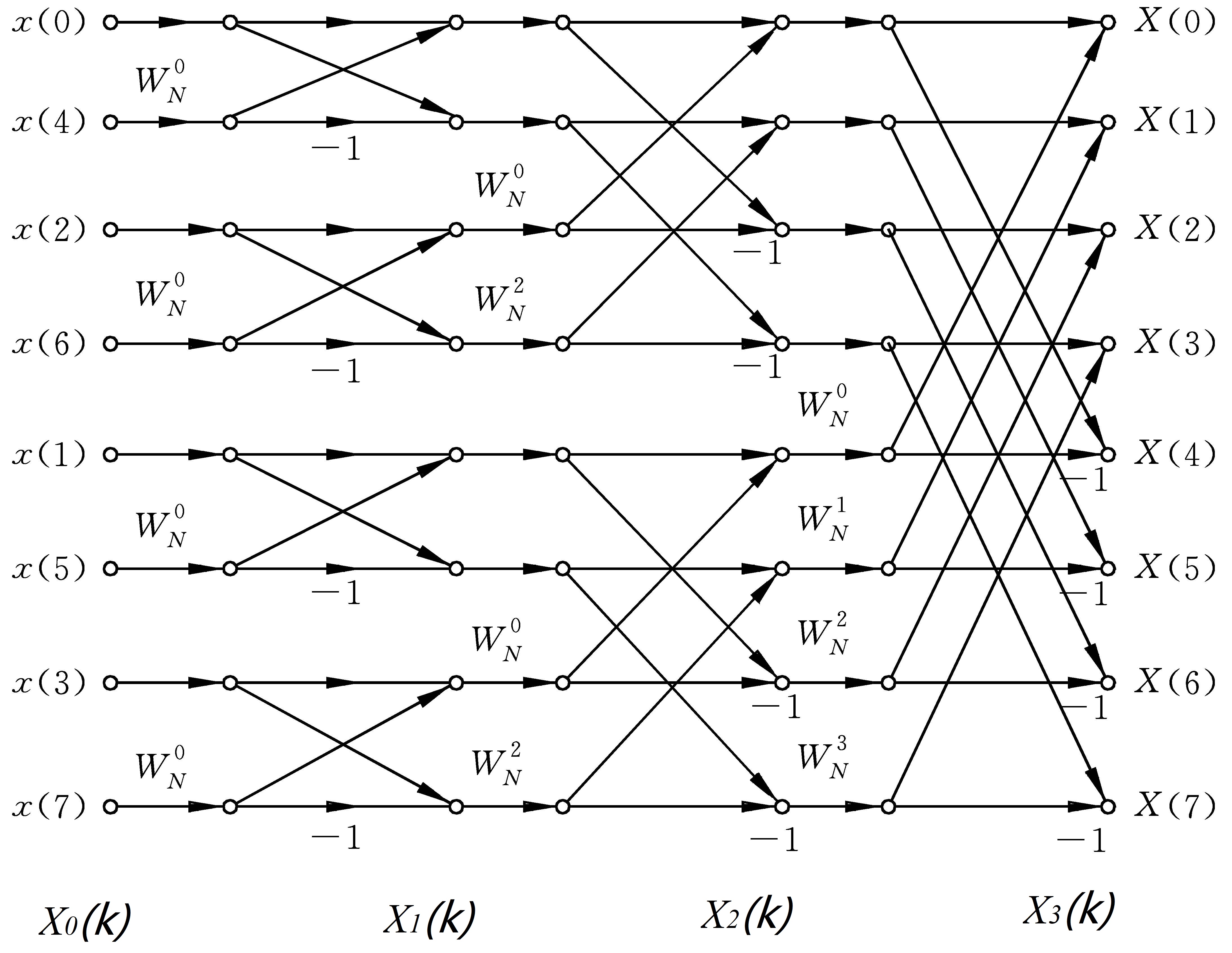
8点FFT计算的结构示意图如下,由图可知,只需要简单的计算几次乘法和加法,便可完成离散傅里叶变换过程,而不是对每个数据进行繁琐的相乘和累加。
 ## 2.3 重要特性
1. **级的概念**
每分割一次,称为一级运算。设FFT运算点数为 $N$ ,共有 $M$ 级运算,则它们满足: $M = log_2^N$
每一级运算的标识为 $m = 0, 1, 2, ..., M-1$ 。
为了便于分割计算,FFT点数 $N$ 的取值经常为2的整数次幂。
2. **蝶形单元**
FFT计算结构由若干个蝶形运算单元组成,每个运算单元示意图如下:
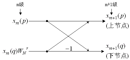
蝶形单元的输入输出满足:
$$
\begin{align}
x_{m+1}(p) = x_{m}(p) + x_{m}(q) \cdot W_N^r \\
x_{m+1}(q) = x_{m}(p) - x_{m}(q) \cdot W_N^r
\end{align}
$$
其中, $q = p + 2^m$ , $W_N^r = cos(\frac{2\pi r}{N}) - jsin(\frac{2\pi r}{N})$
每一个蝶形单元运算时,进行了一次乘法和两次加法。
每一级中,均有 $N/2$ 个蝶形单元。
故完成一次FFT所需要的乘法次数和加法次数分别为: $N/2 \cdot log_2N$ , $N \cdot log_2N$
3. 组的概念
每一级 $N/2$ 个蝶形单元可分为若干组,每一组有着相同的结构与 $W_N^r$ 因子分布。
当 $N = 256$ 时,例如:
$m = 0$ 时,可以分为 $N/2 = 128$ 组。
$m = 1$ 时,可以分为 $N/4 = 64$ 组。
$m = M-1$ 时,此时只能分为 1 组。
4. $W_N^r$ 因子分布
$W_{2^{m+1}}^r$ 因子存在于 $m$ 级,其中 $r=0,1,\dots,2^{m}-1$。
在8点FFT第二级运算中,即 $m=1$ ,蝶形运算因子可以化简为: $W_8^0,\ W_8^2\ =>\ W_4^0,\ W_4^1$
5. 码位倒置
对于 $N=8$ 点的FFT计算, $X(0)$ ~ $X(7)$ 位置对应的2进制码为:
`X(000)`,`X(001)`,`X(010)`,`X(011)`,`X(100)`,`X(101)`,`X(110)`,`X(111)`
将其位置的2进制码进行翻转:
`X(000)`,`X(100)`,`X(010)`,`X(110)`,`X(001)`,`X(101)`,`X(011)`,`X(111)`
此时位置对应的10进制为:
`X(0)`,`X(4)`,`X(2)`,`X(6)`,`X(1)`,`X(5)`,`X(3)`,`X(7)`
恰好对应FFT第一级输入数据的顺序。
该特性有利于FFT的编程实现。
## 2.4 IFFT设计
根据以下公式,序列的逆傅里叶变换可以转换为对序列的共轭求傅里叶变换。只需要在输入输出时将虚部取负,并且在每一次蝶形运算完成后将结果右移1位。
$$
\overline{x}(n) = \frac{1}{N}DFT(\overline{X}(K))
$$
# 3. Matlab定点化
## 3.1 生成定点化的旋转因子
旋转因子左移13位,并量化为16bits,代码位于文件`fft_rotate_factor_fixed16.m`:
```matlab
clear all;
clc;
N = 512;
for m = 0 : N/2-1
W(m+1)=complex(cos(2*pi*m/N), -sin(2*pi*m/N));
end
re = real(W);
re = floor(re'*(2^13));
im = imag(W)
im = floor(im'*(2^13));
save('wn_re_512_fixed16.mat', 're'); % 保存实部
save('wn_im_512_fixed16.mat', 'im'); % 保存虚部
fidr = fopen('wn_re_512_fixed16.coe', 'wt');
fidi = fopen('wn_im_512_fixed16.coe', 'wt');
%- standard format
fprintf(fidr, 'MEMORY_INITIALIZATION_RADIX = 10;\n');
fprintf(fidr, 'MEMORY_INITIALIZATION_VECTOR =\n');
fprintf(fidi, 'MEMORY_INITIALIZATION_RADIX = 10;\n');
fprintf(fidi, 'MEMORY_INITIALIZATION_VECTOR =\n');
%- write data in coe file
for i = 1 : 1 : N/2
fprintf(fidr, '%d,\n', re(i));
fprintf(fidi, '%d,\n', im(i));
end
fclose(fidr);
fclose(fidi);
```
## 3.2 蝶形运算单元
代码位于文件`butterfly.m`:
```matlab
function [xn1_re, xn1_im, xn2_re, xn2_im] = butterfly(xm1_re, xm1_im, xm2_re, xm2_im, w_re, w_im)
xn1_re = xm1_re * (2^13) + xm2_re*w_re - (xm2_im*w_im);
xn1_im = xm1_im * (2^13) + xm2_re*w_im + xm2_im*w_re;
xn2_re = xm1_re * (2^13) - (xm2_re*w_re) + xm2_im*w_im;
xn2_im = xm1_im * (2^13) - (xm2_re*w_im) - (xm2_im*w_re);
xn1_re = floor(xn1_re / (2^13)); % 由于旋转因子扩大了 2^13,在这里除以 2^13 进行还原
xn1_im = floor(xn1_im / (2^13));
xn2_re = floor(xn2_re / (2^13));
xn2_im = floor(xn2_im / (2^13));
xn1_re = int16(xn1_re); % 截断为 16 位有符号整数
xn1_im = int16(xn1_im);
xn2_re = int16(xn2_re);
xn2_im = int16(xn2_im);
end
```
## 3.3 蝶形运算控制器
该部分为本设计的关键,作用为生成蝶形运算输入端数据读取、输出端数据写入地址,并产生读写控制信号。该部分控制算法如下,该代码位于文件`fft_radix2.m`:
```matlab
function [Xk] = fft_radix2(xn, N)
% 计算输入信号 xn 的长度 N 所需要的最小2的幂次
M = nextpow2(N);
N_padded = 2^M;
if length(xn) < N_padded
xn = [xn, zeros(1, N_padded - length(xn))]; % 补零
end
n = 1:N_padded;
x = xn(bitrevorder(n-1) + 1); % 位反转
% 从文件中加载512点定点化旋转因子
load('wn_re_512_fixed16.mat', 're');
load('wn_im_512_fixed16.mat', 'im');
W = complex(re, im);
% FFT计算
for m = 1:M % m为级数
for i = 1:2^(M-m) % i为组数
for j = 1:2^(m-1) % j为蝶形在组内的编号
k = (i-1) * 2^m + j;
n_idx = 2^(M-m)*(j-1); % 对于不同的 N,调整索引
% 根据 N 来调整旋转因子的索引
if N == 256
W_idx = n_idx * 2; % 每两个旋转因子取一个
elseif N == 128
W_idx = n_idx * 4; % 每四个旋转因子取一个
elseif N == 64
W_idx = n_idx * 8; % 每八个旋转因子取一个
else
W_idx = n_idx; % 对于 512点,直接使用
end
[T1_re, T1_im, T2_re, T2_im] = butterfly(real(x(k)), imag(x(k)), ...
real(x(k+2^(m-1))), imag(x(k+2^(m-1))), ...
real(W(W_idx+1)), imag(W(W_idx+1)));
if m == 1
% 打印当前 k 和 k+2^(m-1) 的值以及旋转因子 W(W_idx+1)
disp(['x(k): ', num2str(real(x(k))), ' + ', num2str(imag(x(k))), 'i']);
disp(['x(k+2^(m-1)): ', num2str(real(x(k+2^(m-1)))), ' + ', num2str(imag(x(k+2^(m-1)))) , 'i']);
disp(['W(W_idx+1): ', num2str(real(W(W_idx+1))), ' + ', num2str(imag(W(W_idx+1))), 'i']);
end
x(k+2^(m-1)) = complex(T2_re, T2_im);
x(k) = complex(T1_re, T1_im);
if m == 1
disp(['After level ', num2str(m), ' computation for k = ', num2str(k)]);
disp(['x(k): ', num2str(real(x(k))), ' + ', num2str(imag(x(k))), 'i']);
disp(['x(k+2^(m-1)): ', num2str(real(x(k+2^(m-1)))), ' + ', num2str(imag(x(k+2^(m-1)))) , 'i']);
end
end
end
% 每计算完一级,输出 x 的值
% disp(['After level ', num2str(m), ' computation:']);
% disp(x);
end
Xk = x;
end
```
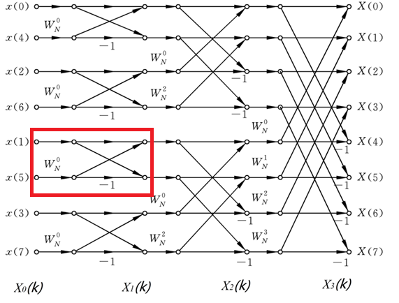
关于各个蝶形单元互联的顺序,256位FFT共有8层,`m`为层数,`i`为组数,`j`为蝶形单元组内编号。可以分析出每个蝶形的输入/出上节点编号,输入/出下节点编号以及旋转因子编号分别为:
输入/出上节点编号: $(i-1)* 2^m + j$
输入/出下节点编号: $(i-1) * 2^m + j + 2^{m-1}$
旋转因子编号: $2^{8-m}*(j-1)$
以下图为例,8位fft共有3层,红框框出的蝶形其层数`m=1`,组数`i=3`,组内编号`j=1`。其上节点编号 $(3-1) \times 2^1+ 1 = 5$ ,即为从上往下数第5个节点(因为输入已经进行了重排,所以这里的编号都是顺序的),下编号节点编号 $5+2^{1-1}=6$ ,旋转因子编号 $2^{3-1} \times (1-1)=0$ ,所以旋转因子是 $W_N^0$ 。
# 4. RTL实现架构
要求实现流水线结构的256位FFT/IFFT运算电路,进行分析有如下要点:
1. FFT/IFFT运算需要在装入全部数据后进行,由于运算电路为串行输入,因此必须要通过`sram`进行装入,待数据全部装入完成后开始运算
2. FFT/IFFT运算结果的输出是**并行同时输出**,由于运算电路为串行输出,因此必须要通过`sram`将**数据由并行转成串行输出**,即结果计算完成后装入`sram`然后依次排出
3. FFT/IFFT运算模块**共用中间的蝶形运算单元阵列**,仅在输入输出处理上有不同,这样方便于减少逻辑资源的消耗。IFFT复用FFT的阵列需要在**输出进行实部和虚部的交换**,以及**实部和虚部需要除以N位**。
**代码实现:**
重排序单元`in_resort.v`:
```verilog
function [8:0] fliplr;
input [8:0] bin;
input [9:0] N;
case(N)
10'd64: fliplr = {bin[8:6],bin[0],bin[1],bin[2],bin[3],bin[4],bin[5]};
10'd128: fliplr = {bin[8:7],bin[0],bin[1],bin[2],bin[3],bin[4],bin[5],bin[6]};
10'd256: fliplr = {bin[8],bin[0],bin[1],bin[2],bin[3],bin[4],bin[5],bin[6],bin[7]};
10'd512: fliplr = {bin[0],bin[1],bin[2],bin[3],bin[4],bin[5],bin[6],bin[7],bin[8]};
default: fliplr = {bin[0],bin[1],bin[2],bin[3],bin[4],bin[5],bin[6],bin[7],bin[8]};
endcase
endfunction
```
蝶形运算单元`butterfly.v`:
```verilog
// ============== 蝶形运算 ===============
// 输入数据延迟一个周期,与权重数据对齐
reg signed [15:0] x1_re_r, x1_im_r;
reg signed [15:0] x2_re_r, x2_im_r;
always @(posedge clk or negedge rst_n) begin
if (!rst_n) begin
x1_re_r <= 16'd0;
x1_im_r <= 16'd0;
x2_re_r <= 16'd0;
x2_im_r <= 16'd0;
end else if (en) begin
x1_re_r <= x1_re;
x1_im_r <= x1_im;
x2_re_r <= x2_re;
x2_im_r <= x2_im;
end
end
reg signed [31:0] y1_re_r, y1_im_r;
reg signed [31:0] y2_re_r, y2_im_r;
always @(*) begin
if (!rst_n) begin
y1_re_r = 32'd0;
y1_im_r = 32'd0;
y2_re_r = 32'd0;
y2_im_r = 32'd0;
end else if (en) begin
y1_re_r = x1_re_r + ((x2_re_r * w_re) >>> 13) - ((x2_im_r * w_im) >>> 13); // 由于 w 被放大了 2^13 倍
y1_im_r = x1_im_r + ((x2_re_r * w_im) >>> 13) + ((x2_im_r * w_re) >>> 13); // 因此需右移 13 位
y2_re_r = x1_re_r - ((x2_re_r * w_re) >>> 13) + ((x2_im_r * w_im) >>> 13);
y2_im_r = x1_im_r - ((x2_re_r * w_im) >>> 13) - ((x2_im_r * w_re) >>> 13);
end
end
assign vld = en_r;
assign y1_re = y1_re_r[15:0];
assign y1_im = y1_im_r[15:0];
assign y2_re = y2_re_r[15:0];
assign y2_im = y2_im_r[15:0];
```
# 5. RTL仿真结果
## 5.1 测试用例说明
将MATLAB中量化后的数据作为输入,将输出写入txt文件中:
```verilog
// 读入数据
initial begin
clk = 1'b1;
rst_n = 1'b0;
inv = 1; // FFT/IFFT
np = 2'b11; // 64/128/256/512
sop_in = 1'b0;
stb = 1'b1;
x_re = 16'd0;
x_im = 16'd0;
cnt0 = 0;
stop_flag = 0;
case(np)
2'b00: N = 10'd64;
2'b01: N = 10'd128;
2'b10: N = 10'd256;
2'b11: N = 10'd512;
endcase
$readmemh("E:/Vivado/fft_pipeline_multimode/fft_pipeline_multimode.srcs/sim_1/new/x_re512.txt", mem_re);
$readmemh("E:/Vivado/fft_pipeline_multimode/fft_pipeline_multimode.srcs/sim_1/new/x_im512.txt", mem_im);
#(period);
rst_n = 1'b1;
#(period);
stb = 1'b0; // 低电平有效
while(cnt0 < N) begin
if(cnt0 == 0)
sop_in = 1;
else
sop_in = 0;
x_re = mem_re[cnt0];
x_im = mem_im[cnt0];
#(period);
cnt0 = cnt0 + 1;
end
stb = 1'b1;
stop_flag = 1;
end
// 写入计算结果
integer cnt1;
initial begin
fdyre = $fopen("E:/Vivado/fft_pipeline_multimode/fft_pipeline_multimode.srcs/sim_1/new/y_ifft512_re.txt", "wb");
fdyim = $fopen("E:/Vivado/fft_pipeline_multimode/fft_pipeline_multimode.srcs/sim_1/new/y_ifft512_im.txt", "wb");
cnt1 = 0;
while(1) begin
if(valid_out == 0) begin
$fwrite(fdyre, "%04x\n", y_re);
$fwrite(fdyim, "%04x\n", y_im);
cnt1 = cnt1 + 1;
end else if(valid_out == 1 && stop_flag == 1 && cnt1 == N) begin
$fclose(fdyre);
$fclose(fdyim);
$stop;
end
#(period);
end
end
```
## 5.2 测试结果波形
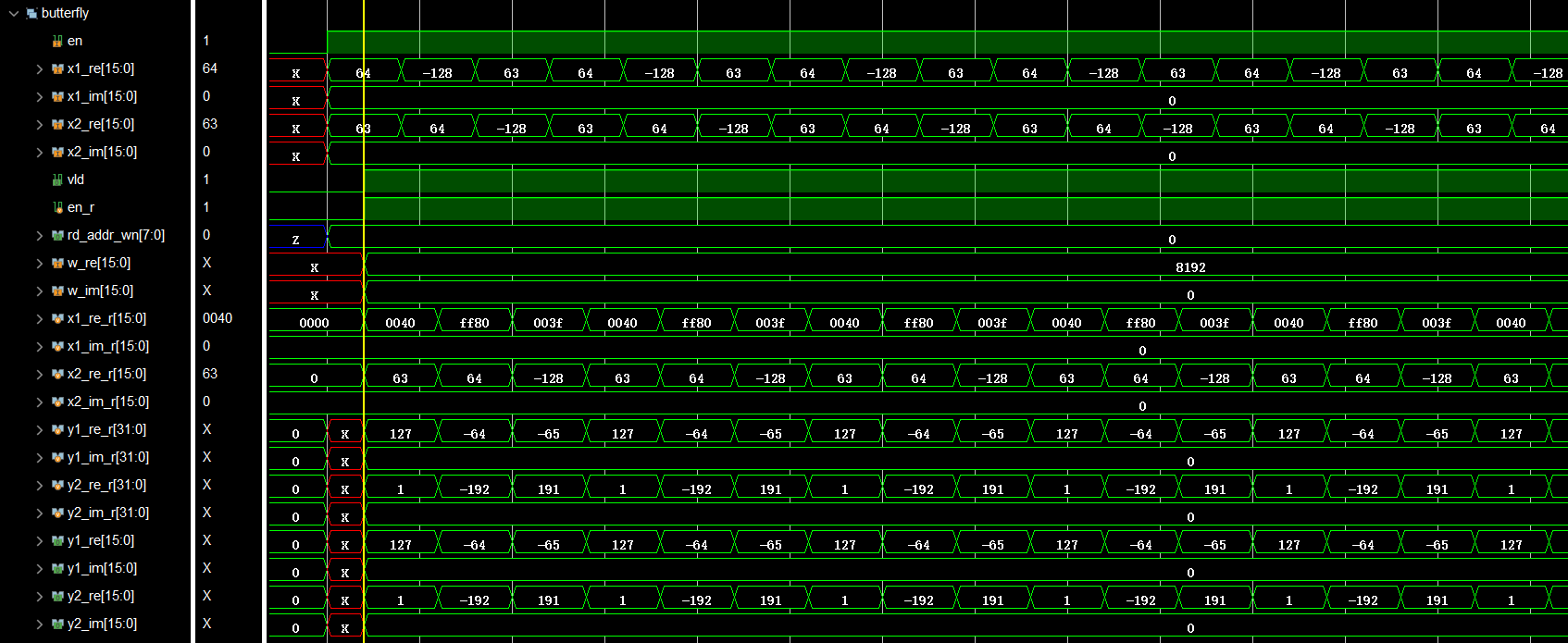
如上图波形可知,该FFT/IFFT单元在正常运行,将输出结果与MATLAB定点化后的模型进行对比:
## 2.3 重要特性
1. **级的概念**
每分割一次,称为一级运算。设FFT运算点数为 $N$ ,共有 $M$ 级运算,则它们满足: $M = log_2^N$
每一级运算的标识为 $m = 0, 1, 2, ..., M-1$ 。
为了便于分割计算,FFT点数 $N$ 的取值经常为2的整数次幂。
2. **蝶形单元**
FFT计算结构由若干个蝶形运算单元组成,每个运算单元示意图如下:

蝶形单元的输入输出满足:
$$
\begin{align}
x_{m+1}(p) = x_{m}(p) + x_{m}(q) \cdot W_N^r \\
x_{m+1}(q) = x_{m}(p) - x_{m}(q) \cdot W_N^r
\end{align}
$$
其中, $q = p + 2^m$ , $W_N^r = cos(\frac{2\pi r}{N}) - jsin(\frac{2\pi r}{N})$
每一个蝶形单元运算时,进行了一次乘法和两次加法。
每一级中,均有 $N/2$ 个蝶形单元。
故完成一次FFT所需要的乘法次数和加法次数分别为: $N/2 \cdot log_2N$ , $N \cdot log_2N$
3. 组的概念
每一级 $N/2$ 个蝶形单元可分为若干组,每一组有着相同的结构与 $W_N^r$ 因子分布。
当 $N = 256$ 时,例如:
$m = 0$ 时,可以分为 $N/2 = 128$ 组。
$m = 1$ 时,可以分为 $N/4 = 64$ 组。
$m = M-1$ 时,此时只能分为 1 组。
4. $W_N^r$ 因子分布
$W_{2^{m+1}}^r$ 因子存在于 $m$ 级,其中 $r=0,1,\dots,2^{m}-1$。
在8点FFT第二级运算中,即 $m=1$ ,蝶形运算因子可以化简为: $W_8^0,\ W_8^2\ =>\ W_4^0,\ W_4^1$
5. 码位倒置
对于 $N=8$ 点的FFT计算, $X(0)$ ~ $X(7)$ 位置对应的2进制码为:
`X(000)`,`X(001)`,`X(010)`,`X(011)`,`X(100)`,`X(101)`,`X(110)`,`X(111)`
将其位置的2进制码进行翻转:
`X(000)`,`X(100)`,`X(010)`,`X(110)`,`X(001)`,`X(101)`,`X(011)`,`X(111)`
此时位置对应的10进制为:
`X(0)`,`X(4)`,`X(2)`,`X(6)`,`X(1)`,`X(5)`,`X(3)`,`X(7)`
恰好对应FFT第一级输入数据的顺序。
该特性有利于FFT的编程实现。
## 2.4 IFFT设计
根据以下公式,序列的逆傅里叶变换可以转换为对序列的共轭求傅里叶变换。只需要在输入输出时将虚部取负,并且在每一次蝶形运算完成后将结果右移1位。
$$
\overline{x}(n) = \frac{1}{N}DFT(\overline{X}(K))
$$
# 3. Matlab定点化
## 3.1 生成定点化的旋转因子
旋转因子左移13位,并量化为16bits,代码位于文件`fft_rotate_factor_fixed16.m`:
```matlab
clear all;
clc;
N = 512;
for m = 0 : N/2-1
W(m+1)=complex(cos(2*pi*m/N), -sin(2*pi*m/N));
end
re = real(W);
re = floor(re'*(2^13));
im = imag(W)
im = floor(im'*(2^13));
save('wn_re_512_fixed16.mat', 're'); % 保存实部
save('wn_im_512_fixed16.mat', 'im'); % 保存虚部
fidr = fopen('wn_re_512_fixed16.coe', 'wt');
fidi = fopen('wn_im_512_fixed16.coe', 'wt');
%- standard format
fprintf(fidr, 'MEMORY_INITIALIZATION_RADIX = 10;\n');
fprintf(fidr, 'MEMORY_INITIALIZATION_VECTOR =\n');
fprintf(fidi, 'MEMORY_INITIALIZATION_RADIX = 10;\n');
fprintf(fidi, 'MEMORY_INITIALIZATION_VECTOR =\n');
%- write data in coe file
for i = 1 : 1 : N/2
fprintf(fidr, '%d,\n', re(i));
fprintf(fidi, '%d,\n', im(i));
end
fclose(fidr);
fclose(fidi);
```
## 3.2 蝶形运算单元
代码位于文件`butterfly.m`:
```matlab
function [xn1_re, xn1_im, xn2_re, xn2_im] = butterfly(xm1_re, xm1_im, xm2_re, xm2_im, w_re, w_im)
xn1_re = xm1_re * (2^13) + xm2_re*w_re - (xm2_im*w_im);
xn1_im = xm1_im * (2^13) + xm2_re*w_im + xm2_im*w_re;
xn2_re = xm1_re * (2^13) - (xm2_re*w_re) + xm2_im*w_im;
xn2_im = xm1_im * (2^13) - (xm2_re*w_im) - (xm2_im*w_re);
xn1_re = floor(xn1_re / (2^13)); % 由于旋转因子扩大了 2^13,在这里除以 2^13 进行还原
xn1_im = floor(xn1_im / (2^13));
xn2_re = floor(xn2_re / (2^13));
xn2_im = floor(xn2_im / (2^13));
xn1_re = int16(xn1_re); % 截断为 16 位有符号整数
xn1_im = int16(xn1_im);
xn2_re = int16(xn2_re);
xn2_im = int16(xn2_im);
end
```
## 3.3 蝶形运算控制器
该部分为本设计的关键,作用为生成蝶形运算输入端数据读取、输出端数据写入地址,并产生读写控制信号。该部分控制算法如下,该代码位于文件`fft_radix2.m`:
```matlab
function [Xk] = fft_radix2(xn, N)
% 计算输入信号 xn 的长度 N 所需要的最小2的幂次
M = nextpow2(N);
N_padded = 2^M;
if length(xn) < N_padded
xn = [xn, zeros(1, N_padded - length(xn))]; % 补零
end
n = 1:N_padded;
x = xn(bitrevorder(n-1) + 1); % 位反转
% 从文件中加载512点定点化旋转因子
load('wn_re_512_fixed16.mat', 're');
load('wn_im_512_fixed16.mat', 'im');
W = complex(re, im);
% FFT计算
for m = 1:M % m为级数
for i = 1:2^(M-m) % i为组数
for j = 1:2^(m-1) % j为蝶形在组内的编号
k = (i-1) * 2^m + j;
n_idx = 2^(M-m)*(j-1); % 对于不同的 N,调整索引
% 根据 N 来调整旋转因子的索引
if N == 256
W_idx = n_idx * 2; % 每两个旋转因子取一个
elseif N == 128
W_idx = n_idx * 4; % 每四个旋转因子取一个
elseif N == 64
W_idx = n_idx * 8; % 每八个旋转因子取一个
else
W_idx = n_idx; % 对于 512点,直接使用
end
[T1_re, T1_im, T2_re, T2_im] = butterfly(real(x(k)), imag(x(k)), ...
real(x(k+2^(m-1))), imag(x(k+2^(m-1))), ...
real(W(W_idx+1)), imag(W(W_idx+1)));
if m == 1
% 打印当前 k 和 k+2^(m-1) 的值以及旋转因子 W(W_idx+1)
disp(['x(k): ', num2str(real(x(k))), ' + ', num2str(imag(x(k))), 'i']);
disp(['x(k+2^(m-1)): ', num2str(real(x(k+2^(m-1)))), ' + ', num2str(imag(x(k+2^(m-1)))) , 'i']);
disp(['W(W_idx+1): ', num2str(real(W(W_idx+1))), ' + ', num2str(imag(W(W_idx+1))), 'i']);
end
x(k+2^(m-1)) = complex(T2_re, T2_im);
x(k) = complex(T1_re, T1_im);
if m == 1
disp(['After level ', num2str(m), ' computation for k = ', num2str(k)]);
disp(['x(k): ', num2str(real(x(k))), ' + ', num2str(imag(x(k))), 'i']);
disp(['x(k+2^(m-1)): ', num2str(real(x(k+2^(m-1)))), ' + ', num2str(imag(x(k+2^(m-1)))) , 'i']);
end
end
end
% 每计算完一级,输出 x 的值
% disp(['After level ', num2str(m), ' computation:']);
% disp(x);
end
Xk = x;
end
```
关于各个蝶形单元互联的顺序,256位FFT共有8层,`m`为层数,`i`为组数,`j`为蝶形单元组内编号。可以分析出每个蝶形的输入/出上节点编号,输入/出下节点编号以及旋转因子编号分别为:
输入/出上节点编号: $(i-1)* 2^m + j$
输入/出下节点编号: $(i-1) * 2^m + j + 2^{m-1}$
旋转因子编号: $2^{8-m}*(j-1)$
以下图为例,8位fft共有3层,红框框出的蝶形其层数`m=1`,组数`i=3`,组内编号`j=1`。其上节点编号 $(3-1) \times 2^1+ 1 = 5$ ,即为从上往下数第5个节点(因为输入已经进行了重排,所以这里的编号都是顺序的),下编号节点编号 $5+2^{1-1}=6$ ,旋转因子编号 $2^{3-1} \times (1-1)=0$ ,所以旋转因子是 $W_N^0$ 。

# 4. RTL实现架构
要求实现流水线结构的256位FFT/IFFT运算电路,进行分析有如下要点:
1. FFT/IFFT运算需要在装入全部数据后进行,由于运算电路为串行输入,因此必须要通过`sram`进行装入,待数据全部装入完成后开始运算
2. FFT/IFFT运算结果的输出是**并行同时输出**,由于运算电路为串行输出,因此必须要通过`sram`将**数据由并行转成串行输出**,即结果计算完成后装入`sram`然后依次排出
3. FFT/IFFT运算模块**共用中间的蝶形运算单元阵列**,仅在输入输出处理上有不同,这样方便于减少逻辑资源的消耗。IFFT复用FFT的阵列需要在**输出进行实部和虚部的交换**,以及**实部和虚部需要除以N位**。
**代码实现:**
重排序单元`in_resort.v`:
```verilog
function [8:0] fliplr;
input [8:0] bin;
input [9:0] N;
case(N)
10'd64: fliplr = {bin[8:6],bin[0],bin[1],bin[2],bin[3],bin[4],bin[5]};
10'd128: fliplr = {bin[8:7],bin[0],bin[1],bin[2],bin[3],bin[4],bin[5],bin[6]};
10'd256: fliplr = {bin[8],bin[0],bin[1],bin[2],bin[3],bin[4],bin[5],bin[6],bin[7]};
10'd512: fliplr = {bin[0],bin[1],bin[2],bin[3],bin[4],bin[5],bin[6],bin[7],bin[8]};
default: fliplr = {bin[0],bin[1],bin[2],bin[3],bin[4],bin[5],bin[6],bin[7],bin[8]};
endcase
endfunction
```
蝶形运算单元`butterfly.v`:
```verilog
// ============== 蝶形运算 ===============
// 输入数据延迟一个周期,与权重数据对齐
reg signed [15:0] x1_re_r, x1_im_r;
reg signed [15:0] x2_re_r, x2_im_r;
always @(posedge clk or negedge rst_n) begin
if (!rst_n) begin
x1_re_r <= 16'd0;
x1_im_r <= 16'd0;
x2_re_r <= 16'd0;
x2_im_r <= 16'd0;
end else if (en) begin
x1_re_r <= x1_re;
x1_im_r <= x1_im;
x2_re_r <= x2_re;
x2_im_r <= x2_im;
end
end
reg signed [31:0] y1_re_r, y1_im_r;
reg signed [31:0] y2_re_r, y2_im_r;
always @(*) begin
if (!rst_n) begin
y1_re_r = 32'd0;
y1_im_r = 32'd0;
y2_re_r = 32'd0;
y2_im_r = 32'd0;
end else if (en) begin
y1_re_r = x1_re_r + ((x2_re_r * w_re) >>> 13) - ((x2_im_r * w_im) >>> 13); // 由于 w 被放大了 2^13 倍
y1_im_r = x1_im_r + ((x2_re_r * w_im) >>> 13) + ((x2_im_r * w_re) >>> 13); // 因此需右移 13 位
y2_re_r = x1_re_r - ((x2_re_r * w_re) >>> 13) + ((x2_im_r * w_im) >>> 13);
y2_im_r = x1_im_r - ((x2_re_r * w_im) >>> 13) - ((x2_im_r * w_re) >>> 13);
end
end
assign vld = en_r;
assign y1_re = y1_re_r[15:0];
assign y1_im = y1_im_r[15:0];
assign y2_re = y2_re_r[15:0];
assign y2_im = y2_im_r[15:0];
```
# 5. RTL仿真结果
## 5.1 测试用例说明
将MATLAB中量化后的数据作为输入,将输出写入txt文件中:
```verilog
// 读入数据
initial begin
clk = 1'b1;
rst_n = 1'b0;
inv = 1; // FFT/IFFT
np = 2'b11; // 64/128/256/512
sop_in = 1'b0;
stb = 1'b1;
x_re = 16'd0;
x_im = 16'd0;
cnt0 = 0;
stop_flag = 0;
case(np)
2'b00: N = 10'd64;
2'b01: N = 10'd128;
2'b10: N = 10'd256;
2'b11: N = 10'd512;
endcase
$readmemh("E:/Vivado/fft_pipeline_multimode/fft_pipeline_multimode.srcs/sim_1/new/x_re512.txt", mem_re);
$readmemh("E:/Vivado/fft_pipeline_multimode/fft_pipeline_multimode.srcs/sim_1/new/x_im512.txt", mem_im);
#(period);
rst_n = 1'b1;
#(period);
stb = 1'b0; // 低电平有效
while(cnt0 < N) begin
if(cnt0 == 0)
sop_in = 1;
else
sop_in = 0;
x_re = mem_re[cnt0];
x_im = mem_im[cnt0];
#(period);
cnt0 = cnt0 + 1;
end
stb = 1'b1;
stop_flag = 1;
end
// 写入计算结果
integer cnt1;
initial begin
fdyre = $fopen("E:/Vivado/fft_pipeline_multimode/fft_pipeline_multimode.srcs/sim_1/new/y_ifft512_re.txt", "wb");
fdyim = $fopen("E:/Vivado/fft_pipeline_multimode/fft_pipeline_multimode.srcs/sim_1/new/y_ifft512_im.txt", "wb");
cnt1 = 0;
while(1) begin
if(valid_out == 0) begin
$fwrite(fdyre, "%04x\n", y_re);
$fwrite(fdyim, "%04x\n", y_im);
cnt1 = cnt1 + 1;
end else if(valid_out == 1 && stop_flag == 1 && cnt1 == N) begin
$fclose(fdyre);
$fclose(fdyim);
$stop;
end
#(period);
end
end
```
## 5.2 测试结果波形

如上图波形可知,该FFT/IFFT单元在正常运行,将输出结果与MATLAB定点化后的模型进行对比:
 由上图可知,FFT/IFFT单元输出正确。
# 1. Design Function and Requirements
FFT is used for the fast computation of the Discrete Fourier Transform (DFT). The DFT of a sequence $x(n)$ of length $N$ is defined as:
$$
X(k) = \sum_{n=0}^{N-1} x(n)e^{-j2\pi nk/N}
$$
The corresponding Inverse DFT (IDFT) of the sequence $X(k)$ is defined as:
$$
x(n) = \sum_{n=0}^{N-1} X(k)e^{j2\pi nk/N}
$$
In this definition of DFT and IDFT, the constant factor at the beginning is ignored.
This design involves an FFT processor with sequential logic that supports the computation of 64/128/256/512/1024-point FFT and IFFT. The module is implemented using a pipelined structure and can process multiple consecutive sets of input data.
The top-level module is named `fft_multimode`, and the input/output functionality is defined as follows:
| Name | Direction | Bit Width | Description |
|----------|-----------|-----------|----------------------------------------------------|
| clk | Input | 1 | System clock |
| rst_n | Input | 1 | System asynchronous reset, active low |
| inv | Input | 1 | Mode control, 0 for FFT operation, 1 for IFFT |
| np | Input | 2 | FFT/IFFT point size: 0 for 64-point, 1 for 128-point, 2 for 256-point, 3 for 512-point |
| stb | Input | 1 | Input data valid indication, active low |
| sop_in | Input | 1 | First valid input data indication, active high |
| x_re | Input | 16 | Real part of input data, in 2's complement fixed-point format |
| x_im | Input | 16 | Imaginary part of input data, in 2's complement fixed-point format |
| valid_out| Output | 1 | Output data valid indication, active low |
| sop_out | Output | 1 | First valid output data indication, active low |
| y_re | Output | 16 | Real part of output data, in 2's complement fixed-point format |
| y_im | Output | 16 | Imaginary part of output data, in 2's complement fixed-point format |
**Design Requirements:**
- Matlab floating-point model, fixed-point model;
- Verilog implementation code should be synthesizable, with detailed design documentation, synthesis (performance/area), and simulation results;
- During the processing of each data set, the values of `inv` and `np` signals remain unchanged;
- Support for switching between multiple data sets with different modes (FFT/IFFT, different point sizes);
- Precision control during the computation process to ensure the accuracy of the output. The output fixed-point format (precision range) can be adjusted as needed, with error analysis conducted on the results.
# 2. Algorithm Principles and Design
## 2.1 Formula Derivation
The DFT computation formula is:
$$
X[k]=\sum_{n=0}^{N-1} x[n]W_N^{nk},\ 0 \le k \le N-1
$$
Where, $W_N^{nk} = e^{-j\frac{2\pi k}{N}n}$.
By splitting the DFT formula into odd and even terms, the first $N/2$ points can be expressed as:
$$
\begin{align}
X[k] &= \sum_{r=0}^{\frac{N}{2}-1} X[2r]W_N^{2rk} + \sum_{r=0}^{\frac{N}{2}-1} X[2r+1]W_N^{(2r+1)k}\\
&= \sum_{r=0}^{\frac{N}{2}-1} X[2r]W_{\frac{N}{2}}^{rk} + W_N^k \sum_{r=0}^{\frac{N}{2}-1} X[2r+1]W_{\frac{N}{2}}^{rk}\\
&= A[k] + W_N^k B[k],\ k=0,1,\dots,\frac{N}{2}-1
\end{align}
$$
Similarly, the last $N/2$ points can be expressed as:
$$
\begin{align}
X[k+N/2] &= \sum_{r=0}^{\frac{N}{2}-1} X[2r]W_N^{2r(k+N/2)} + \sum_{r=0}^{\frac{N}{2}-1} X[2r+1]W_N^{(2r+1)(k+N/2)}\\
&= \sum_{r=0}^{\frac{N}{2}-1} X[2r]W_{\frac{N}{2}}^{r(k+N/2)} + W_N^{(k+N/2)} \sum_{r=0}^{\frac{N}{2}-1} X[2r+1]W_{\frac{N}{2}}^{r(k+N/2)}\\
&= \sum_{r=0}^{\frac{N}{2}-1} X[2r]W_{\frac{N}{2}}^{r(k+N/2)} + W_N^{N/2}W_N^k \sum_{r=0}^{\frac{N}{2}-1} X[2r+1]W_{\frac{N}{2}}^{r(k+N/2)}\\
&= \sum_{r=0}^{\frac{N}{2}-1} X[2r]W_{\frac{N}{2}}^{r(k+N/2)} - W_N^k \sum_{r=0}^{\frac{N}{2}-1} X[2r+1]W_{\frac{N}{2}}^{r(k+N/2)}\\
&= A[k] - W_N^k B[k],\ k=0,1,\dots,\frac{N}{2}-1
\end{align}
$$
Where, $W_N^{N/2}W_N^k = -W_N^k$, and $W_N^k = \cos\left(\frac{2\pi k}{N}\right) - j\sin\left(\frac{2\pi k}{N}\right)$.
Thus, the values of the last $N/2$ points can be fully determined by the intermediate values computed during the calculation of the first $N/2$ points. By recursively applying even-odd decomposition to $A[k]$ and $B[k]$ until the DFT becomes a 2-point DFT, many redundant calculations can be avoided, leading to the efficient computation of FFT.
## 2.2 Algorithm Structure
The structure diagram of an 8-point FFT computation is shown below. From the diagram, we can see that only a few multiplications and additions are required to complete the Discrete Fourier Transform, rather than performing cumbersome multiplications and summations for each data point.
## 2.3 Important Characteristics
1. **Concept of Levels**
Each division is called a level of computation. Let the FFT point size be $N$, and the total number of levels be $M$. They satisfy the relation: $M = \log_2 N$.
Each level of computation is identified as $m = 0, 1, 2, ..., M-1$.
For ease of computation, the FFT point size $N$ is often a power of 2.
2. **Butterfly Unit**
The FFT computation structure consists of several butterfly computation units. The schematic diagram of each butterfly unit is as follows:

The input-output relationships of the butterfly unit are:
$$
\begin{align}
x_{m+1}(p) = x_{m}(p) + x_{m}(q) \cdot W_N^r \\
x_{m+1}(q) = x_{m}(p) - x_{m}(q) \cdot W_N^r
\end{align}
$$
Where, $q = p + 2^m$, and $W_N^r = \cos\left(\frac{2\pi r}{N}\right) - j\sin\left(\frac{2\pi r}{N}\right)$.
Each butterfly unit operation involves one multiplication and two additions.
Each level contains $N/2$ butterfly units.
Therefore, the number of multiplications and additions required for completing one FFT is $N/2 \cdot \log_2 N$ and $N \cdot \log_2 N$, respectively.
3. **Concept of Groups**
Each level of $N/2$ butterfly units can be divided into several groups, each with the same structure and $W_N^r$ factor distribution.
When $N = 256$, for example:
- For $m = 0$, there are $N/2 = 128$ groups.
- For $m = 1$, there are $N/4 = 64$ groups.
- For $m = M-1$, there is only 1 group.
4. **$W_N^r$ Factor Distribution**
The $W_{2^{m+1}}^r$ factors exist in the $m$-th level, where $r = 0,1,\dots,2^m - 1$.
In the second level of the 8-point FFT (i.e., $m=1$), the butterfly operation factors simplify to: $W_8^0,\ W_8^2 \Rightarrow W_4^0,\ W_4^1$.
5. **Bit Reversal**
For an $N=8$-point FFT computation, the binary positions of $X(0)$ to $X(7)$ are:
`X(000)`, `X(001)`, `X(010)`, `X(011)`, `X(100)`, `X(101)`, `X(110)`, `X(111)`.
Reversing their binary codes gives:
`X(000)`, `X(100)`, `X(010)`, `X(110)`, `X(001)`, `X(101)`, `X(011)`, `X(111)`.
Corresponding decimal positions are:
`X(0)`, `X(4)`, `X(2)`, `X(6)`, `X(1)`, `X(5)`, `X(3)`, `X(7)`.
This reversal corresponds exactly to the order of input data in the first level of the FFT.
This feature is beneficial for FFT programming implementation.
## 2.4 IFFT Design
Based on the following formula, the Inverse Fourier Transform (IFFT) of a sequence can be converted into a Fourier transform of the conjugate of the sequence. The imaginary part is negated during input/output, and the result is right-shifted by one bit after each butterfly computation:
$$
\overline{x}(n) = \frac{1}{N}DFT(\overline{X}(K))
$$
# 3. Fixed-Point Implementation in Matlab
## 3.1 Generating Fixed-Point Rotation Factors
The rotation factors are left-shifted by 13 bits and quantized to 16 bits. The code is located in the file `fft_rotate_factor_fixed16.m`:
```matlab
clear all;
clc;
N = 512;
for m = 0 : N/2-1
W(m+1)=complex(cos(2*pi*m/N), -sin(2*pi*m/N));
end
re = real(W);
re = floor(re'*(2^13));
im = imag(W)
im = floor(im'*(2^13));
save('wn_re_512_fixed16.mat', 're'); % Save real part
save('wn_im_512_fixed16.mat', 'im'); % Save imaginary part
fidr = fopen('wn_re_512_fixed16.coe', 'wt');
fidi = fopen('wn_im_512_fixed16.coe', 'wt');
%- standard format
fprintf(fidr, 'MEMORY_INITIALIZATION_RADIX = 10;\n');
fprintf(fidr, 'MEMORY_INITIALIZATION_VECTOR =\n');
fprintf(fidi, 'MEMORY_INITIALIZATION_RADIX = 10;\n');
fprintf(fidi, 'MEMORY_INITIALIZATION_VECTOR =\n');
%- write data in coe file
for i = 1 : 1 : N/2
fprintf(fidr, '%d,\n', re(i));
fprintf(fidi, '%d,\n', im(i));
end
fclose(fidr);
fclose(fidi);
```
## 3.2 Butterfly Operation Unit
The code is located in the file `butterfly.m`:
```matlab
function [xn1_re, xn1_im, xn2_re, xn2_im] = butterfly(xm1_re, xm1_im, xm2_re, xm2_im, w_re, w_im)
xn1_re = xm1_re * (2^13) + xm2_re*w_re - (xm2_im*w_im);
xn1_im = xm1_im * (2^13) + xm2_re*w_im + xm2_im*w_re;
xn2_re = xm1_re * (2^13) - (xm2_re*w_re) + xm2_im*w_im;
xn2_im = xm1_im * (2^13) - (xm2_re*w_im) - (xm2_im*w_re);
xn1_re = floor(xn1_re / (2^13)); % Since the rotation factor is scaled by 2^13, divide by 2^13 to undo scaling
xn1_im = floor(xn1_im / (2^13));
xn2_re = floor(xn2_re / (2^13));
xn2_im = floor(xn2_im / (2^13));
xn1_re = int16(xn1_re); % Truncate to 16-bit signed integer
xn1_im = int16(xn1_im);
xn2_re = int16(xn2_re);
xn2_im = int16(xn2_im);
end
```
## 3.3 Butterfly Operation Controller
This part is key to the design, and its function is to generate the input data read addresses, output data write addresses, and control signals for reading and writing. The control algorithm for this section is as follows, and the code is located in the file `fft_radix2.m`:
```matlab
function [Xk] = fft_radix2(xn, N)
% Calculate the smallest power of 2 required for the input signal length xn
M = nextpow2(N);
N_padded = 2^M;
if length(xn) < N_padded
xn = [xn, zeros(1, N_padded - length(xn))]; % Zero-padding
end
n = 1:N_padded;
x = xn(bitrevorder(n-1) + 1); % Bit-reversal
% Load fixed-point 512-point rotation factors from file
load('wn_re_512_fixed16.mat', 're');
load('wn_im_512_fixed16.mat', 'im');
W = complex(re, im);
% FFT calculation
for m = 1:M % m is the stage number
for i = 1:2^(M-m) % i is the group number
for j = 1:2^(m-1) % j is the butterfly unit number within the group
k = (i-1) * 2^m + j;
n_idx = 2^(M-m)*(j-1); % Adjust index for different N
% Adjust the rotation factor index based on N
if N == 256
W_idx = n_idx * 2; % Take one rotation factor for every two
elseif N == 128
W_idx = n_idx * 4; % Take one rotation factor for every four
elseif N == 64
W_idx = n_idx * 8; % Take one rotation factor for every eight
else
W_idx = n_idx; % For 512-point, use directly
end
[T1_re, T1_im, T2_re, T2_im] = butterfly(real(x(k)), imag(x(k)), ...
real(x(k+2^(m-1))), imag(x(k+2^(m-1))), ...
real(W(W_idx+1)), imag(W(W_idx+1)));
if m == 1
% Display current values of k and k+2^(m-1) and rotation factor W(W_idx+1)
disp(['x(k): ', num2str(real(x(k))), ' + ', num2str(imag(x(k))), 'i']);
disp(['x(k+2^(m-1)): ', num2str(real(x(k+2^(m-1)))), ' + ', num2str(imag(x(k+2^(m-1)))) , 'i']);
disp(['W(W_idx+1): ', num2str(real(W(W_idx+1))), ' + ', num2str(imag(W(W_idx+1))), 'i']);
end
x(k+2^(m-1)) = complex(T2_re, T2_im);
x(k) = complex(T1_re, T1_im);
if m == 1
disp(['After level ', num2str(m), ' computation for k = ', num2str(k)]);
disp(['x(k): ', num2str(real(x(k))), ' + ', num2str(imag(x(k))), 'i']);
disp(['x(k+2^(m-1)): ', num2str(real(x(k+2^(m-1)))), ' + ', num2str(imag(x(k+2^(m-1)))) , 'i']);
end
end
end
% Output x after each stage computation
% disp(['After level ', num2str(m), ' computation:']);
% disp(x);
end
Xk = x;
end
```
The interconnection sequence of the butterfly units in the 256-point FFT consists of 8 stages. Here, `m` is the stage number, `i` is the group number, and `j` is the butterfly unit number within the group. We can analyze the input/output node numbers for each butterfly unit, the corresponding node numbers for the input/output, and the rotation factor index as follows:
Input/Output Upper Node Number: $(i-1)* 2^m + j$
Input/Output Lower Node Number: $(i-1) * 2^m + j + 2^{m-1}$
Rotation Factor Index: $2^{8-m}*(j-1)$
The following figure shows an example for an 8-point FFT with 3 stages. The butterfly highlighted in red has stage `m=1`, group number `i=3`, and group number within the group `j=1`. Its upper node number is $(3-1)2^1 + 1 = 5$, meaning it's the 5th node from the top (since the input is reordered, the numbering here is sequential). The lower node number is $5+2^{1-1} = 6$, and the rotation factor index is $2^{3-1}(1-1) = 0$, so the rotation factor is $W_N^0$.

# 4. RTL Implementation Architecture
The goal is to implement a 256-bit FFT/IFFT computation circuit with a pipelined structure. The key points for analysis are as follows:
1. The FFT/IFFT computation must begin after all data has been loaded. Since the computation circuit has serial input, it is necessary to load the data through `sram`. Once the data is completely loaded, the computation can start.
2. The FFT/IFFT computation results are **parallel and simultaneous outputs**. Since the computation circuit has serial output, it is necessary to use `sram` to **convert the parallel data into serial output**. That is, once the computation is completed, the results are loaded into `sram` and then sequentially released.
3. The FFT/IFFT computation module **shares the intermediate butterfly computation unit array**, with only the input and output processing differing. This helps reduce logic resource consumption. The IFFT reuses the FFT array but requires **swapping the real and imaginary parts** in the output, and the **real and imaginary parts need to be divided by N**.
**Code Implementation:**
Reordering Unit `in_resort.v`:
```verilog
function [8:0] fliplr;
input [8:0] bin;
input [9:0] N;
case(N)
10'd64: fliplr = {bin[8:6],bin[0],bin[1],bin[2],bin[3],bin[4],bin[5]};
10'd128: fliplr = {bin[8:7],bin[0],bin[1],bin[2],bin[3],bin[4],bin[5],bin[6]};
10'd256: fliplr = {bin[8],bin[0],bin[1],bin[2],bin[3],bin[4],bin[5],bin[6],bin[7]};
10'd512: fliplr = {bin[0],bin[1],bin[2],bin[3],bin[4],bin[5],bin[6],bin[7],bin[8]};
default: fliplr = {bin[0],bin[1],bin[2],bin[3],bin[4],bin[5],bin[6],bin[7],bin[8]};
endcase
endfunction
```
Butterfly Computation Unit `butterfly.v`:
```verilog
// ============== Butterfly Computation ===============
// Input data is delayed by one cycle to align with the weight data
reg signed [15:0] x1_re_r, x1_im_r;
reg signed [15:0] x2_re_r, x2_im_r;
always @(posedge clk or negedge rst_n) begin
if (!rst_n) begin
x1_re_r <= 16'd0;
x1_im_r <= 16'd0;
x2_re_r <= 16'd0;
x2_im_r <= 16'd0;
end else if (en) begin
x1_re_r <= x1_re;
x1_im_r <= x1_im;
x2_re_r <= x2_re;
x2_im_r <= x2_im;
end
end
reg signed [31:0] y1_re_r, y1_im_r;
reg signed [31:0] y2_re_r, y2_im_r;
always @(*) begin
if (!rst_n) begin
y1_re_r = 32'd0;
y1_im_r = 32'd0;
y2_re_r = 32'd0;
y2_im_r = 32'd0;
end else if (en) begin
y1_re_r = x1_re_r + ((x2_re_r * w_re) >>> 13) - ((x2_im_r * w_im) >>> 13); // Since w is scaled by 2^13, right shift by 13
y1_im_r = x1_im_r + ((x2_re_r * w_im) >>> 13) + ((x2_im_r * w_re) >>> 13); // Thus, right shift by 13
y2_re_r = x1_re_r - ((x2_re_r * w_re) >>> 13) + ((x2_im_r * w_im) >>> 13);
y2_im_r = x1_im_r - ((x2_re_r * w_im) >>> 13) - ((x2_im_r * w_re) >>> 13);
end
end
assign vld = en_r;
assign y1_re = y1_re_r[15:0];
assign y1_im = y1_im_r[15:0];
assign y2_re = y2_re_r[15:0];
assign y2_im = y2_im_r[15:0];
```
# 5. RTL Simulation Results
## 5.1 Test Case Description
The quantized data from MATLAB is used as input, and the output is written to a txt file:
```verilog
// Read in data
initial begin
clk = 1'b1;
rst_n = 1'b0;
inv = 1; // FFT/IFFT
np = 2'b11; // 64/128/256/512
sop_in = 1'b0;
stb = 1'b1;
x_re = 16'd0;
x_im = 16'd0;
cnt0 = 0;
stop_flag = 0;
case(np)
2'b00: N = 10'd64;
2'b01: N = 10'd128;
2'b10: N = 10'd256;
2'b11: N = 10'd512;
endcase
$readmemh("E:/Vivado/fft_pipeline_multimode/fft_pipeline_multimode.srcs/sim_1/new/x_re512.txt", mem_re);
$readmemh("E:/Vivado/fft_pipeline_multimode/fft_pipeline_multimode.srcs/sim_1/new/x_im512.txt", mem_im);
#(period);
rst_n = 1'b1;
#(period);
stb = 1'b0; // Active low
while(cnt0 < N) begin
if(cnt0 == 0)
sop_in = 1;
else
sop_in = 0;
x_re = mem_re[cnt0];
x_im = mem_im[cnt0];
#(period);
cnt0 = cnt0 + 1;
end
stb = 1'b1;
stop_flag = 1;
end
// Write computation results
integer cnt1;
initial begin
fdyre = $fopen("E:/Vivado/fft_pipeline_multimode/fft_pipeline_multimode.srcs/sim_1/new/y_ifft512_re.txt", "wb");
fdyim = $fopen("E:/Vivado/fft_pipeline_multimode/fft_pipeline_multimode.srcs/sim_1/new/y_ifft512_im.txt", "wb");
cnt1 = 0;
while(1) begin
if(valid_out == 0) begin
$fwrite(fdyre, "%04x\n", y_re);
$fwrite(fdyim, "%04x\n", y_im);
cnt1 = cnt1 + 1;
end else if(valid_out == 1 && stop_flag == 1 && cnt1 == N) begin
$fclose(fdyre);
$fclose(fdyim);
$stop;
end
#(period);
end
end
```
## 5.2 Test Waveform Results

As shown in the waveform above, the FFT/IFFT unit operates correctly. The output results are compared with the fixed-point MATLAB model:
From the above images, we can see that the FFT/IFFT unit outputs correctly.
由上图可知,FFT/IFFT单元输出正确。
# 1. Design Function and Requirements
FFT is used for the fast computation of the Discrete Fourier Transform (DFT). The DFT of a sequence $x(n)$ of length $N$ is defined as:
$$
X(k) = \sum_{n=0}^{N-1} x(n)e^{-j2\pi nk/N}
$$
The corresponding Inverse DFT (IDFT) of the sequence $X(k)$ is defined as:
$$
x(n) = \sum_{n=0}^{N-1} X(k)e^{j2\pi nk/N}
$$
In this definition of DFT and IDFT, the constant factor at the beginning is ignored.
This design involves an FFT processor with sequential logic that supports the computation of 64/128/256/512/1024-point FFT and IFFT. The module is implemented using a pipelined structure and can process multiple consecutive sets of input data.
The top-level module is named `fft_multimode`, and the input/output functionality is defined as follows:
| Name | Direction | Bit Width | Description |
|----------|-----------|-----------|----------------------------------------------------|
| clk | Input | 1 | System clock |
| rst_n | Input | 1 | System asynchronous reset, active low |
| inv | Input | 1 | Mode control, 0 for FFT operation, 1 for IFFT |
| np | Input | 2 | FFT/IFFT point size: 0 for 64-point, 1 for 128-point, 2 for 256-point, 3 for 512-point |
| stb | Input | 1 | Input data valid indication, active low |
| sop_in | Input | 1 | First valid input data indication, active high |
| x_re | Input | 16 | Real part of input data, in 2's complement fixed-point format |
| x_im | Input | 16 | Imaginary part of input data, in 2's complement fixed-point format |
| valid_out| Output | 1 | Output data valid indication, active low |
| sop_out | Output | 1 | First valid output data indication, active low |
| y_re | Output | 16 | Real part of output data, in 2's complement fixed-point format |
| y_im | Output | 16 | Imaginary part of output data, in 2's complement fixed-point format |
**Design Requirements:**
- Matlab floating-point model, fixed-point model;
- Verilog implementation code should be synthesizable, with detailed design documentation, synthesis (performance/area), and simulation results;
- During the processing of each data set, the values of `inv` and `np` signals remain unchanged;
- Support for switching between multiple data sets with different modes (FFT/IFFT, different point sizes);
- Precision control during the computation process to ensure the accuracy of the output. The output fixed-point format (precision range) can be adjusted as needed, with error analysis conducted on the results.
# 2. Algorithm Principles and Design
## 2.1 Formula Derivation
The DFT computation formula is:
$$
X[k]=\sum_{n=0}^{N-1} x[n]W_N^{nk},\ 0 \le k \le N-1
$$
Where, $W_N^{nk} = e^{-j\frac{2\pi k}{N}n}$.
By splitting the DFT formula into odd and even terms, the first $N/2$ points can be expressed as:
$$
\begin{align}
X[k] &= \sum_{r=0}^{\frac{N}{2}-1} X[2r]W_N^{2rk} + \sum_{r=0}^{\frac{N}{2}-1} X[2r+1]W_N^{(2r+1)k}\\
&= \sum_{r=0}^{\frac{N}{2}-1} X[2r]W_{\frac{N}{2}}^{rk} + W_N^k \sum_{r=0}^{\frac{N}{2}-1} X[2r+1]W_{\frac{N}{2}}^{rk}\\
&= A[k] + W_N^k B[k],\ k=0,1,\dots,\frac{N}{2}-1
\end{align}
$$
Similarly, the last $N/2$ points can be expressed as:
$$
\begin{align}
X[k+N/2] &= \sum_{r=0}^{\frac{N}{2}-1} X[2r]W_N^{2r(k+N/2)} + \sum_{r=0}^{\frac{N}{2}-1} X[2r+1]W_N^{(2r+1)(k+N/2)}\\
&= \sum_{r=0}^{\frac{N}{2}-1} X[2r]W_{\frac{N}{2}}^{r(k+N/2)} + W_N^{(k+N/2)} \sum_{r=0}^{\frac{N}{2}-1} X[2r+1]W_{\frac{N}{2}}^{r(k+N/2)}\\
&= \sum_{r=0}^{\frac{N}{2}-1} X[2r]W_{\frac{N}{2}}^{r(k+N/2)} + W_N^{N/2}W_N^k \sum_{r=0}^{\frac{N}{2}-1} X[2r+1]W_{\frac{N}{2}}^{r(k+N/2)}\\
&= \sum_{r=0}^{\frac{N}{2}-1} X[2r]W_{\frac{N}{2}}^{r(k+N/2)} - W_N^k \sum_{r=0}^{\frac{N}{2}-1} X[2r+1]W_{\frac{N}{2}}^{r(k+N/2)}\\
&= A[k] - W_N^k B[k],\ k=0,1,\dots,\frac{N}{2}-1
\end{align}
$$
Where, $W_N^{N/2}W_N^k = -W_N^k$, and $W_N^k = \cos\left(\frac{2\pi k}{N}\right) - j\sin\left(\frac{2\pi k}{N}\right)$.
Thus, the values of the last $N/2$ points can be fully determined by the intermediate values computed during the calculation of the first $N/2$ points. By recursively applying even-odd decomposition to $A[k]$ and $B[k]$ until the DFT becomes a 2-point DFT, many redundant calculations can be avoided, leading to the efficient computation of FFT.
## 2.2 Algorithm Structure
The structure diagram of an 8-point FFT computation is shown below. From the diagram, we can see that only a few multiplications and additions are required to complete the Discrete Fourier Transform, rather than performing cumbersome multiplications and summations for each data point.
## 2.3 Important Characteristics
1. **Concept of Levels**
Each division is called a level of computation. Let the FFT point size be $N$, and the total number of levels be $M$. They satisfy the relation: $M = \log_2 N$.
Each level of computation is identified as $m = 0, 1, 2, ..., M-1$.
For ease of computation, the FFT point size $N$ is often a power of 2.
2. **Butterfly Unit**
The FFT computation structure consists of several butterfly computation units. The schematic diagram of each butterfly unit is as follows:

The input-output relationships of the butterfly unit are:
$$
\begin{align}
x_{m+1}(p) = x_{m}(p) + x_{m}(q) \cdot W_N^r \\
x_{m+1}(q) = x_{m}(p) - x_{m}(q) \cdot W_N^r
\end{align}
$$
Where, $q = p + 2^m$, and $W_N^r = \cos\left(\frac{2\pi r}{N}\right) - j\sin\left(\frac{2\pi r}{N}\right)$.
Each butterfly unit operation involves one multiplication and two additions.
Each level contains $N/2$ butterfly units.
Therefore, the number of multiplications and additions required for completing one FFT is $N/2 \cdot \log_2 N$ and $N \cdot \log_2 N$, respectively.
3. **Concept of Groups**
Each level of $N/2$ butterfly units can be divided into several groups, each with the same structure and $W_N^r$ factor distribution.
When $N = 256$, for example:
- For $m = 0$, there are $N/2 = 128$ groups.
- For $m = 1$, there are $N/4 = 64$ groups.
- For $m = M-1$, there is only 1 group.
4. **$W_N^r$ Factor Distribution**
The $W_{2^{m+1}}^r$ factors exist in the $m$-th level, where $r = 0,1,\dots,2^m - 1$.
In the second level of the 8-point FFT (i.e., $m=1$), the butterfly operation factors simplify to: $W_8^0,\ W_8^2 \Rightarrow W_4^0,\ W_4^1$.
5. **Bit Reversal**
For an $N=8$-point FFT computation, the binary positions of $X(0)$ to $X(7)$ are:
`X(000)`, `X(001)`, `X(010)`, `X(011)`, `X(100)`, `X(101)`, `X(110)`, `X(111)`.
Reversing their binary codes gives:
`X(000)`, `X(100)`, `X(010)`, `X(110)`, `X(001)`, `X(101)`, `X(011)`, `X(111)`.
Corresponding decimal positions are:
`X(0)`, `X(4)`, `X(2)`, `X(6)`, `X(1)`, `X(5)`, `X(3)`, `X(7)`.
This reversal corresponds exactly to the order of input data in the first level of the FFT.
This feature is beneficial for FFT programming implementation.
## 2.4 IFFT Design
Based on the following formula, the Inverse Fourier Transform (IFFT) of a sequence can be converted into a Fourier transform of the conjugate of the sequence. The imaginary part is negated during input/output, and the result is right-shifted by one bit after each butterfly computation:
$$
\overline{x}(n) = \frac{1}{N}DFT(\overline{X}(K))
$$
# 3. Fixed-Point Implementation in Matlab
## 3.1 Generating Fixed-Point Rotation Factors
The rotation factors are left-shifted by 13 bits and quantized to 16 bits. The code is located in the file `fft_rotate_factor_fixed16.m`:
```matlab
clear all;
clc;
N = 512;
for m = 0 : N/2-1
W(m+1)=complex(cos(2*pi*m/N), -sin(2*pi*m/N));
end
re = real(W);
re = floor(re'*(2^13));
im = imag(W)
im = floor(im'*(2^13));
save('wn_re_512_fixed16.mat', 're'); % Save real part
save('wn_im_512_fixed16.mat', 'im'); % Save imaginary part
fidr = fopen('wn_re_512_fixed16.coe', 'wt');
fidi = fopen('wn_im_512_fixed16.coe', 'wt');
%- standard format
fprintf(fidr, 'MEMORY_INITIALIZATION_RADIX = 10;\n');
fprintf(fidr, 'MEMORY_INITIALIZATION_VECTOR =\n');
fprintf(fidi, 'MEMORY_INITIALIZATION_RADIX = 10;\n');
fprintf(fidi, 'MEMORY_INITIALIZATION_VECTOR =\n');
%- write data in coe file
for i = 1 : 1 : N/2
fprintf(fidr, '%d,\n', re(i));
fprintf(fidi, '%d,\n', im(i));
end
fclose(fidr);
fclose(fidi);
```
## 3.2 Butterfly Operation Unit
The code is located in the file `butterfly.m`:
```matlab
function [xn1_re, xn1_im, xn2_re, xn2_im] = butterfly(xm1_re, xm1_im, xm2_re, xm2_im, w_re, w_im)
xn1_re = xm1_re * (2^13) + xm2_re*w_re - (xm2_im*w_im);
xn1_im = xm1_im * (2^13) + xm2_re*w_im + xm2_im*w_re;
xn2_re = xm1_re * (2^13) - (xm2_re*w_re) + xm2_im*w_im;
xn2_im = xm1_im * (2^13) - (xm2_re*w_im) - (xm2_im*w_re);
xn1_re = floor(xn1_re / (2^13)); % Since the rotation factor is scaled by 2^13, divide by 2^13 to undo scaling
xn1_im = floor(xn1_im / (2^13));
xn2_re = floor(xn2_re / (2^13));
xn2_im = floor(xn2_im / (2^13));
xn1_re = int16(xn1_re); % Truncate to 16-bit signed integer
xn1_im = int16(xn1_im);
xn2_re = int16(xn2_re);
xn2_im = int16(xn2_im);
end
```
## 3.3 Butterfly Operation Controller
This part is key to the design, and its function is to generate the input data read addresses, output data write addresses, and control signals for reading and writing. The control algorithm for this section is as follows, and the code is located in the file `fft_radix2.m`:
```matlab
function [Xk] = fft_radix2(xn, N)
% Calculate the smallest power of 2 required for the input signal length xn
M = nextpow2(N);
N_padded = 2^M;
if length(xn) < N_padded
xn = [xn, zeros(1, N_padded - length(xn))]; % Zero-padding
end
n = 1:N_padded;
x = xn(bitrevorder(n-1) + 1); % Bit-reversal
% Load fixed-point 512-point rotation factors from file
load('wn_re_512_fixed16.mat', 're');
load('wn_im_512_fixed16.mat', 'im');
W = complex(re, im);
% FFT calculation
for m = 1:M % m is the stage number
for i = 1:2^(M-m) % i is the group number
for j = 1:2^(m-1) % j is the butterfly unit number within the group
k = (i-1) * 2^m + j;
n_idx = 2^(M-m)*(j-1); % Adjust index for different N
% Adjust the rotation factor index based on N
if N == 256
W_idx = n_idx * 2; % Take one rotation factor for every two
elseif N == 128
W_idx = n_idx * 4; % Take one rotation factor for every four
elseif N == 64
W_idx = n_idx * 8; % Take one rotation factor for every eight
else
W_idx = n_idx; % For 512-point, use directly
end
[T1_re, T1_im, T2_re, T2_im] = butterfly(real(x(k)), imag(x(k)), ...
real(x(k+2^(m-1))), imag(x(k+2^(m-1))), ...
real(W(W_idx+1)), imag(W(W_idx+1)));
if m == 1
% Display current values of k and k+2^(m-1) and rotation factor W(W_idx+1)
disp(['x(k): ', num2str(real(x(k))), ' + ', num2str(imag(x(k))), 'i']);
disp(['x(k+2^(m-1)): ', num2str(real(x(k+2^(m-1)))), ' + ', num2str(imag(x(k+2^(m-1)))) , 'i']);
disp(['W(W_idx+1): ', num2str(real(W(W_idx+1))), ' + ', num2str(imag(W(W_idx+1))), 'i']);
end
x(k+2^(m-1)) = complex(T2_re, T2_im);
x(k) = complex(T1_re, T1_im);
if m == 1
disp(['After level ', num2str(m), ' computation for k = ', num2str(k)]);
disp(['x(k): ', num2str(real(x(k))), ' + ', num2str(imag(x(k))), 'i']);
disp(['x(k+2^(m-1)): ', num2str(real(x(k+2^(m-1)))), ' + ', num2str(imag(x(k+2^(m-1)))) , 'i']);
end
end
end
% Output x after each stage computation
% disp(['After level ', num2str(m), ' computation:']);
% disp(x);
end
Xk = x;
end
```
The interconnection sequence of the butterfly units in the 256-point FFT consists of 8 stages. Here, `m` is the stage number, `i` is the group number, and `j` is the butterfly unit number within the group. We can analyze the input/output node numbers for each butterfly unit, the corresponding node numbers for the input/output, and the rotation factor index as follows:
Input/Output Upper Node Number: $(i-1)* 2^m + j$
Input/Output Lower Node Number: $(i-1) * 2^m + j + 2^{m-1}$
Rotation Factor Index: $2^{8-m}*(j-1)$
The following figure shows an example for an 8-point FFT with 3 stages. The butterfly highlighted in red has stage `m=1`, group number `i=3`, and group number within the group `j=1`. Its upper node number is $(3-1)2^1 + 1 = 5$, meaning it's the 5th node from the top (since the input is reordered, the numbering here is sequential). The lower node number is $5+2^{1-1} = 6$, and the rotation factor index is $2^{3-1}(1-1) = 0$, so the rotation factor is $W_N^0$.

# 4. RTL Implementation Architecture
The goal is to implement a 256-bit FFT/IFFT computation circuit with a pipelined structure. The key points for analysis are as follows:
1. The FFT/IFFT computation must begin after all data has been loaded. Since the computation circuit has serial input, it is necessary to load the data through `sram`. Once the data is completely loaded, the computation can start.
2. The FFT/IFFT computation results are **parallel and simultaneous outputs**. Since the computation circuit has serial output, it is necessary to use `sram` to **convert the parallel data into serial output**. That is, once the computation is completed, the results are loaded into `sram` and then sequentially released.
3. The FFT/IFFT computation module **shares the intermediate butterfly computation unit array**, with only the input and output processing differing. This helps reduce logic resource consumption. The IFFT reuses the FFT array but requires **swapping the real and imaginary parts** in the output, and the **real and imaginary parts need to be divided by N**.
**Code Implementation:**
Reordering Unit `in_resort.v`:
```verilog
function [8:0] fliplr;
input [8:0] bin;
input [9:0] N;
case(N)
10'd64: fliplr = {bin[8:6],bin[0],bin[1],bin[2],bin[3],bin[4],bin[5]};
10'd128: fliplr = {bin[8:7],bin[0],bin[1],bin[2],bin[3],bin[4],bin[5],bin[6]};
10'd256: fliplr = {bin[8],bin[0],bin[1],bin[2],bin[3],bin[4],bin[5],bin[6],bin[7]};
10'd512: fliplr = {bin[0],bin[1],bin[2],bin[3],bin[4],bin[5],bin[6],bin[7],bin[8]};
default: fliplr = {bin[0],bin[1],bin[2],bin[3],bin[4],bin[5],bin[6],bin[7],bin[8]};
endcase
endfunction
```
Butterfly Computation Unit `butterfly.v`:
```verilog
// ============== Butterfly Computation ===============
// Input data is delayed by one cycle to align with the weight data
reg signed [15:0] x1_re_r, x1_im_r;
reg signed [15:0] x2_re_r, x2_im_r;
always @(posedge clk or negedge rst_n) begin
if (!rst_n) begin
x1_re_r <= 16'd0;
x1_im_r <= 16'd0;
x2_re_r <= 16'd0;
x2_im_r <= 16'd0;
end else if (en) begin
x1_re_r <= x1_re;
x1_im_r <= x1_im;
x2_re_r <= x2_re;
x2_im_r <= x2_im;
end
end
reg signed [31:0] y1_re_r, y1_im_r;
reg signed [31:0] y2_re_r, y2_im_r;
always @(*) begin
if (!rst_n) begin
y1_re_r = 32'd0;
y1_im_r = 32'd0;
y2_re_r = 32'd0;
y2_im_r = 32'd0;
end else if (en) begin
y1_re_r = x1_re_r + ((x2_re_r * w_re) >>> 13) - ((x2_im_r * w_im) >>> 13); // Since w is scaled by 2^13, right shift by 13
y1_im_r = x1_im_r + ((x2_re_r * w_im) >>> 13) + ((x2_im_r * w_re) >>> 13); // Thus, right shift by 13
y2_re_r = x1_re_r - ((x2_re_r * w_re) >>> 13) + ((x2_im_r * w_im) >>> 13);
y2_im_r = x1_im_r - ((x2_re_r * w_im) >>> 13) - ((x2_im_r * w_re) >>> 13);
end
end
assign vld = en_r;
assign y1_re = y1_re_r[15:0];
assign y1_im = y1_im_r[15:0];
assign y2_re = y2_re_r[15:0];
assign y2_im = y2_im_r[15:0];
```
# 5. RTL Simulation Results
## 5.1 Test Case Description
The quantized data from MATLAB is used as input, and the output is written to a txt file:
```verilog
// Read in data
initial begin
clk = 1'b1;
rst_n = 1'b0;
inv = 1; // FFT/IFFT
np = 2'b11; // 64/128/256/512
sop_in = 1'b0;
stb = 1'b1;
x_re = 16'd0;
x_im = 16'd0;
cnt0 = 0;
stop_flag = 0;
case(np)
2'b00: N = 10'd64;
2'b01: N = 10'd128;
2'b10: N = 10'd256;
2'b11: N = 10'd512;
endcase
$readmemh("E:/Vivado/fft_pipeline_multimode/fft_pipeline_multimode.srcs/sim_1/new/x_re512.txt", mem_re);
$readmemh("E:/Vivado/fft_pipeline_multimode/fft_pipeline_multimode.srcs/sim_1/new/x_im512.txt", mem_im);
#(period);
rst_n = 1'b1;
#(period);
stb = 1'b0; // Active low
while(cnt0 < N) begin
if(cnt0 == 0)
sop_in = 1;
else
sop_in = 0;
x_re = mem_re[cnt0];
x_im = mem_im[cnt0];
#(period);
cnt0 = cnt0 + 1;
end
stb = 1'b1;
stop_flag = 1;
end
// Write computation results
integer cnt1;
initial begin
fdyre = $fopen("E:/Vivado/fft_pipeline_multimode/fft_pipeline_multimode.srcs/sim_1/new/y_ifft512_re.txt", "wb");
fdyim = $fopen("E:/Vivado/fft_pipeline_multimode/fft_pipeline_multimode.srcs/sim_1/new/y_ifft512_im.txt", "wb");
cnt1 = 0;
while(1) begin
if(valid_out == 0) begin
$fwrite(fdyre, "%04x\n", y_re);
$fwrite(fdyim, "%04x\n", y_im);
cnt1 = cnt1 + 1;
end else if(valid_out == 1 && stop_flag == 1 && cnt1 == N) begin
$fclose(fdyre);
$fclose(fdyim);
$stop;
end
#(period);
end
end
```
## 5.2 Test Waveform Results

As shown in the waveform above, the FFT/IFFT unit operates correctly. The output results are compared with the fixed-point MATLAB model:
From the above images, we can see that the FFT/IFFT unit outputs correctly.