# PyL7Plot
**Repository Path**: lvisei/PyL7Plot
## Basic Information
- **Project Name**: PyL7Plot
- **Description**: 🌍 Python3 binding for @AntV/L7Plot Plotting Library
- **Primary Language**: Unknown
- **License**: MIT
- **Default Branch**: main
- **Homepage**: None
- **GVP Project**: No
## Statistics
- **Stars**: 0
- **Forks**: 0
- **Created**: 2022-06-15
- **Last Updated**: 2022-06-15
## Categories & Tags
**Categories**: Uncategorized
**Tags**: None
## README
 [English](./README.md) | 简体中文
# PyL7Plot
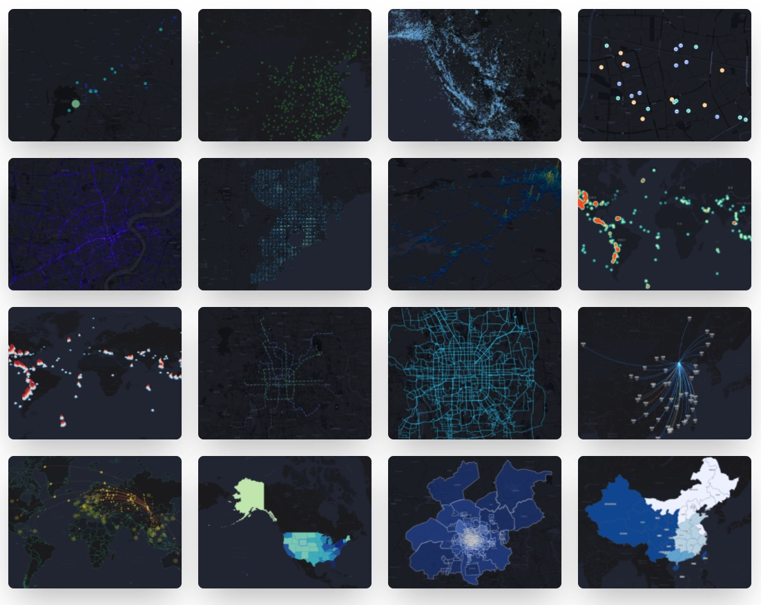
🌍 PyL7Plot 是 [`@AntV/L7Plot`](https://github.com/antvis/L7Plot) 在 Python3 上的封装。L7Plot 是基于 L7 的地理空间可视化图表库。
[](https://pypi.python.org/pypi/pyl7plot)
[](https://github.com/lvisei/pyl7plot/actions?query=workflow%3Abuild)
[](https://pypi.python.org/pypi/pyl7plot)
## 安装
```bash
$ pip install pyl7plot
```
## 使用
#### **渲染成 HTML**
```py
from pyl7plot import Plot
dot = Plot("Dot")
dot.set_options({
"map": {
"type": "mapbox",
"style": "light",
"center": [103.447303, 31.753574],
"zoom": 7,
},
"autoFit": True,
"source": {
"data": [
{ "lng": 103.715, "lat": 31.211, "depth": 10, "mag": 5.8, "title": "M 5.8 - eastern Sichuan, China" },
{ "lng": 104.682, "lat": 31.342, "depth": 10, "mag": 5.7, "title": "M 5.7 - eastern Sichuan, China" },
# ...
],
"parser": { "type": "json", "x": "lng", "y": "lat" },
},
"color": {
"field": "mag",
"value": ["#82cf9c", "#10b3b0", "#2033ab"],
"scale": { "type": "quantize" },
},
"size": {
"field": "mag",
},
"state": { "active": True },
"scale": { "position": "bottomright" },
"legend": { "position": "bottomleft" },
"tooltip": {
"items": ["title", "mag", "depth"],
},
})
# 渲染成 html 文件
dot.render("dot.html")
# 或者渲染成 html 字符串
# dot.render_html()
```

#### **在 Jupyter 中使用**
```py
from pyl7plot import Plot, JS
dot = Plot("Dot")
dot.set_options({
"map": {
"type": "mapbox",
"style": "light",
"center": [103.447303, 31.753574],
"zoom": 7,
},
"autoFit": True,
"height": 400, # 设置在 jupyter 预览的高度
"source": {
"data": [
{ "lng": 103.715, "lat": 31.211, "depth": 10, "mag": 5.8, "title": "M 5.8 - eastern Sichuan, China" },
{ "lng": 104.682, "lat": 31.342, "depth": 10, "mag": 5.7, "title": "M 5.7 - eastern Sichuan, China" },
# ...
],
"parser": { "type": "json", "x": "lng", "y": "lat" },
},
"color": {
"field": "mag",
"value": ["#82cf9c", "#10b3b0", "#2033ab"],
"scale": { "type": "quantize" },
},
"size": {
"field": "mag",
# 使用 JS 方法,可以创建一个 JavaScript 的代码片段去处理各种回调方法属性
"value": JS('''function({ mag }) {
return (mag - 4.3) * 10;
}''')
},
"state": { "active": True },
"scale": { "position": "bottomright" },
"legend": { "position": "bottomleft" },
"tooltip": {
"items": ["title", "mag", "depth"],
},
})
# 渲染到 notebook
dot.render_notebook()
# 或者渲染到 jupyter lab
# dot.render_jupyter_lab()
```
> 更多 PyL7plot 在线 [Jupyter Lab](https://colab.research.google.com/drive/11gTHsZ5Xg31jjJUJWEt5PkZv0VE9qyAG?usp=sharing) 示例。
## API
- **Plot**
1. _Plot(plot_type: str)_: 获取 `Plot` 对应的类实例。
2. _plot.set_options(options: object)_: 给图表实例设置一个 [L7Plot](https://l7plot.antv.vision/) 图形的配置,文档可以直接参考 L7Plot 官网,未进行任何二次数据结构包装。
3. _plot.render(path, env, \*\*kwargs)_: 渲染出一个 HTML 文件,同时可以传入文件的路径,以及 jinja2 env 和 kwargs 参数。
4. _plot.render_notebook(env, \*\*kwargs)_: 将图表渲染到 jupyter 的预览。
5. _plot.render_jupyter_lab(env, \*\*kwargs)_: 将图表渲染到 jupyter lab 的预览。
6. _plot.render_html(env, \*\*kwargs)_: 渲染出 HTML 字符串,同时可以传入 jinja2 env 和 kwargs 参数。
## 协议
[MIT](./LICENSE)
[English](./README.md) | 简体中文
# PyL7Plot
🌍 PyL7Plot 是 [`@AntV/L7Plot`](https://github.com/antvis/L7Plot) 在 Python3 上的封装。L7Plot 是基于 L7 的地理空间可视化图表库。
[](https://pypi.python.org/pypi/pyl7plot)
[](https://github.com/lvisei/pyl7plot/actions?query=workflow%3Abuild)
[](https://pypi.python.org/pypi/pyl7plot)
## 安装
```bash
$ pip install pyl7plot
```
## 使用
#### **渲染成 HTML**
```py
from pyl7plot import Plot
dot = Plot("Dot")
dot.set_options({
"map": {
"type": "mapbox",
"style": "light",
"center": [103.447303, 31.753574],
"zoom": 7,
},
"autoFit": True,
"source": {
"data": [
{ "lng": 103.715, "lat": 31.211, "depth": 10, "mag": 5.8, "title": "M 5.8 - eastern Sichuan, China" },
{ "lng": 104.682, "lat": 31.342, "depth": 10, "mag": 5.7, "title": "M 5.7 - eastern Sichuan, China" },
# ...
],
"parser": { "type": "json", "x": "lng", "y": "lat" },
},
"color": {
"field": "mag",
"value": ["#82cf9c", "#10b3b0", "#2033ab"],
"scale": { "type": "quantize" },
},
"size": {
"field": "mag",
},
"state": { "active": True },
"scale": { "position": "bottomright" },
"legend": { "position": "bottomleft" },
"tooltip": {
"items": ["title", "mag", "depth"],
},
})
# 渲染成 html 文件
dot.render("dot.html")
# 或者渲染成 html 字符串
# dot.render_html()
```

#### **在 Jupyter 中使用**
```py
from pyl7plot import Plot, JS
dot = Plot("Dot")
dot.set_options({
"map": {
"type": "mapbox",
"style": "light",
"center": [103.447303, 31.753574],
"zoom": 7,
},
"autoFit": True,
"height": 400, # 设置在 jupyter 预览的高度
"source": {
"data": [
{ "lng": 103.715, "lat": 31.211, "depth": 10, "mag": 5.8, "title": "M 5.8 - eastern Sichuan, China" },
{ "lng": 104.682, "lat": 31.342, "depth": 10, "mag": 5.7, "title": "M 5.7 - eastern Sichuan, China" },
# ...
],
"parser": { "type": "json", "x": "lng", "y": "lat" },
},
"color": {
"field": "mag",
"value": ["#82cf9c", "#10b3b0", "#2033ab"],
"scale": { "type": "quantize" },
},
"size": {
"field": "mag",
# 使用 JS 方法,可以创建一个 JavaScript 的代码片段去处理各种回调方法属性
"value": JS('''function({ mag }) {
return (mag - 4.3) * 10;
}''')
},
"state": { "active": True },
"scale": { "position": "bottomright" },
"legend": { "position": "bottomleft" },
"tooltip": {
"items": ["title", "mag", "depth"],
},
})
# 渲染到 notebook
dot.render_notebook()
# 或者渲染到 jupyter lab
# dot.render_jupyter_lab()
```
> 更多 PyL7plot 在线 [Jupyter Lab](https://colab.research.google.com/drive/11gTHsZ5Xg31jjJUJWEt5PkZv0VE9qyAG?usp=sharing) 示例。
## API
- **Plot**
1. _Plot(plot_type: str)_: 获取 `Plot` 对应的类实例。
2. _plot.set_options(options: object)_: 给图表实例设置一个 [L7Plot](https://l7plot.antv.vision/) 图形的配置,文档可以直接参考 L7Plot 官网,未进行任何二次数据结构包装。
3. _plot.render(path, env, \*\*kwargs)_: 渲染出一个 HTML 文件,同时可以传入文件的路径,以及 jinja2 env 和 kwargs 参数。
4. _plot.render_notebook(env, \*\*kwargs)_: 将图表渲染到 jupyter 的预览。
5. _plot.render_jupyter_lab(env, \*\*kwargs)_: 将图表渲染到 jupyter lab 的预览。
6. _plot.render_html(env, \*\*kwargs)_: 渲染出 HTML 字符串,同时可以传入 jinja2 env 和 kwargs 参数。
## 协议
[MIT](./LICENSE)